Your first PINN in the Lab: the 1D Poisson equation

This guide solves the 1D Poisson equation. By the end you will have built a complete physics-informed neural network (PINN) in the Lab without writing any code, downloaded the PyTorch script it generates, trained it, and shown that its answer matches the exact solution to about four or five digits.

Poisson is the right first problem: it has one unknown function, one variable, no time, and an exact answer you can write on a napkin. Everything you learn here (domain, equation, conditions, network, loss, optimiser, training) carries over unchanged to harder problems.

Before you start. Open the Lab and choose an empty canvas. If you would rather see a finished example first, open the Poisson on a square notebook, which is the same idea in two dimensions, and come back here.

1. The problem

We want a function $u(x)$ on the interval $0 < x < 1$ that satisfies

$$ -\frac{d^2 u}{dx^2} = f(x), \qquad f(x) = \pi^2 \sin(\pi x), $$

and is pinned to zero at both ends:

$$ u(0) = 0, \qquad u(1) = 0 . $$

Physically you can read this as the steady temperature of a thin bar that is held at zero degrees at both ends and heated along its length by a source $f(x)$. The first equation is the governing equation, the other two are the boundary conditions. Together they pick out exactly one solution.

The exact answer (so we can check ourselves)

Try $u(x) = \sin(\pi x)$. Differentiating twice gives $u'' = -\pi^2 \sin(\pi x)$, so $-u'' = \pi^2\sin(\pi x) = f(x)$, and $\sin(0) = \sin(\pi) = 0$ satisfies both boundary conditions. So

$$ u_{\text{exact}}(x) = \sin(\pi x). $$

A PINN never sees this formula during training. We keep it only to grade the result.

2. How a PINN sees the problem

A PINN replaces the unknown function with a neural network $u_\theta(x)$, where $\theta$ are the network's weights. It is not shown any answers. It is shown how wrong it currently is, in two ways.

The equation error. Pick points $x_1,\dots,x_{N_r}$ inside the interval (the collocation points). At each one, differentiate the network twice with automatic differentiation and measure how far the equation is from holding:

$$ r_\theta(x) = -\frac{d^2 u_\theta}{dx^2}(x) - f(x). $$

If $u_\theta$ were the true solution, $r_\theta$ would be zero everywhere. It is called the residual.

The boundary error. At the two ends, the network should output zero:

$$ u_\theta(0) = 0, \qquad u_\theta(1) = 0 . $$

Training pushes both errors down together by minimising one number, the loss:

$$ \mathcal{L}(\theta) \;=\; \underbrace{\frac{1}{N_r}\sum_{i=1}^{N_r} r_\theta(x_i)^2}_{\text{PDE loss}} \;+\; \underbrace{\frac{1}{N_b}\sum_{j=1}^{N_b} u_\theta(x_j^{b})^2}_{\text{boundary loss}} . $$

When both terms are close to zero, the network satisfies the equation at the sample points and the boundary conditions, and, because the problem has a unique solution, it must be close to the true $u$ in between.

Why $\tanh$ and not ReLU? The residual contains a second derivative of the network. A ReLU network is piecewise linear, so its second derivative is zero almost everywhere and the equation error carries no information. Smooth activations such as $\tanh$ have meaningful second derivatives. Use a smooth activation for any PDE with second-order terms.

3. The plan: one block per decision

The Lab turns each ingredient of the maths above into a block. You set them in this order, and the Lab checks the wiring as you connect them.

#	Block	The question it answers	Our choice
1	DOM Domain	Where does the problem live?	One space dimension, $x \in [0, 1]$, no time
2	PDE Equation	Which equation must hold inside?	Poisson, $-u'' = f$, with $f = \pi^2\sin(\pi x)$
3	BC Boundary	What is fixed at the edges?	$u(0)=0$ and $u(1)=0$
4	NET Network	What function family do we search in?	1 input, 3 hidden layers of 32 neurons, $\tanh$, 1 output
5	LOSS Loss	How do we score the errors?	Mean squared error, PDE and boundary weights both 1
6	OPT Optimiser	How do the weights change?	Adam, learning rate $10^{-3}$
7	RUN Train	How long and with how many points?	5000 epochs, 100 interior points

A note on labels. The Lab's wording can differ slightly between versions (for example "Equation" versus "PDE"). The quantity to set is what matters; if a field name here does not match the screen exactly, pick the nearest one. If a value is not offered, keep the Lab's default and carry on.

4. Step by step in the Lab

Step 1: Domain (DOM)

Add a Domain block. Make it one-dimensional, with the single coordinate $x$ running from 0 to 1. Leave time switched off. This problem is steady, so nothing changes in time.

Check: the block shows one coordinate and no time axis.

Step 2: Equation (PDE)

Add an Equation block and connect it to the Domain. Choose the Poisson equation. If the Lab asks for the source term, enter

$$ f(x) = \pi^2 \sin(\pi x) $$

in whatever syntax the field uses (typically pi**2 * sin(pi*x) or pi^2*sin(pi*x)). Be careful about the sign: the equation is $-u'' = f$, which is the same as $u'' = -f$. A flipped sign is the most common reason a first run returns a mirror image of the right answer.

Check: the block's summary reads as the equation above, with the same $f$.

Step 3: Boundary conditions (BC)

Add a Boundary block and connect it to the Domain. You need two conditions, one at each end of the interval:

Where	Type	Value
$x = 0$	Fixed value (Dirichlet)	$u = 0$
$x = 1$	Fixed value (Dirichlet)	$u = 0$

A Dirichlet condition fixes the value of $u$ itself. (The other common kind, Neumann, fixes the slope $u'$, and appears in later guides.)

Check: the Lab counts two boundary conditions. A 1D interval has exactly two ends, and the Lab warns you if the count does not match what the equation needs.

Step 4: Network (NET)

Add a Network block. It has one input ($x$) and one output ($u$). For the hidden part use 3 layers of 32 neurons with the tanh activation.

Do not agonise over these numbers. For a problem this smooth, anything from 2 layers of 16 neurons upward works. Bigger networks are slower and not necessarily better.

Check: the Lab fills in the input and output sizes for you from the Domain and Equation blocks. If you see a warning about a mismatch, it is almost always a wrong input size.

Step 5: Loss (LOSS)

Add a Loss block and connect the Equation, Boundary and Network blocks to it. Use mean squared error for both the PDE and the boundary terms, and set both weights to 1.

This is exactly the loss $\mathcal{L}$ from Section 2. The weights decide how much each kind of error matters. They are the first thing to adjust if a run misbehaves (see Troubleshooting below).

Check: the Loss block lists two terms, "PDE" and "Boundary".

Step 6: Optimiser (OPT)

Add an Optimiser block. Choose Adam with a learning rate of 0.001 (written 1e-3). Adam is the standard first choice: it copes well with the noisy, badly scaled gradients that PINN losses produce.

Step 7: Train (RUN)

Add the Train block and connect the Loss and Optimiser to it. Set 5000 epochs and 100 interior collocation points (the Lab places the two boundary points for you).

Check: the Lab shows no warnings. If it shows some, fix the flagged block before going on. A clean check means the configuration is consistent, not that the answer will be accurate. Only the comparison in Step 9 tells you that.

Step 8: Generate and run

1. Click the button that generates the Python code and download the script. You may be asked for your name, email, affiliation and intended use first.
2. Install PyTorch if you do not have it: pip install torch.
3. Run the script: python your_script.py.

Remember: the Lab builds and checks the configuration, but it does not train the model. Training happens on your own computer, in the script you downloaded.

While it trains you should see the loss printed at intervals. On an ordinary laptop 5000 epochs of this size takes well under a minute.

Step 9: Judge the result

Training finishing is not the same as the answer being right. Check three things.

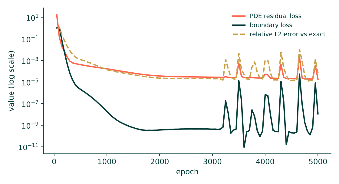
1. Did the loss fall? It should drop by several orders of magnitude, from tens at the start to around $10^{-4}$ or $10^{-5}$.

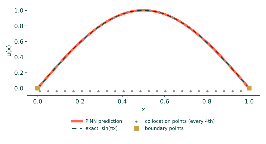
2. Does the curve look right? Plot the network's prediction against the exact $\sin(\pi x)$. They should be almost indistinguishable.

3. How big is the error? The pointwise error should be tiny everywhere, with no large bump near the ends.

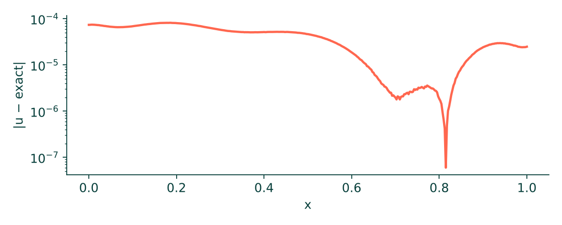
The measure we use is the relative $L^2$ error against the exact solution,

$$ \varepsilon = \frac{\lVert u_\theta - u_{\text{exact}} \rVert_2}{\lVert u_{\text{exact}} \rVert_2}, $$

evaluated on a fine grid that is different from the training points. Checking on points the network trained on would flatter it.

What to expect

These figures come from a hand-written reference implementation with exactly the settings above (random seed 0). Your numbers will differ, because the Lab's script may initialise and sample slightly differently, but you should land in the same neighbourhood.

Epoch	Total loss	Relative $L^2$ error
0	$5 \times 10^{1}$	$1.2$
500	$4 \times 10^{-4}$	$1.2 \times 10^{-3}$
1000	$2 \times 10^{-4}$	$1.4 \times 10^{-4}$
2000	$4 \times 10^{-5}$	$2.3 \times 10^{-5}$
5000	$2 \times 10^{-5}$	$7 \times 10^{-5}$

The largest pointwise error at the end was about $8 \times 10^{-5}$.

Do not worry about spikes. In the reference run the error briefly jumped by about two orders of magnitude near epoch 3500 and then recovered within a few hundred epochs. That is ordinary behaviour for Adam on a PINN loss. Judge a run by where it settles, not by one noisy moment. If you have the choice, keep the best result, not the last.

5. If something goes wrong

What you see	Likely cause	What to try
The curve is the right shape but upside down	Sign of the source term	Re-read Step 2: the equation is $-u'' = f$
The ends of the curve do not reach zero	Boundary term is too weak next to the PDE term	Raise the boundary weight to 10 or 100 and rerun
Loss stalls around $10^{-1}$ or higher	Network too small, learning rate too high, or too few points	Try 3 × 32 with learning rate $10^{-3}$; raise points to 200
Loss is nan	Learning rate far too high, or a typo in $f$	Lower the rate to $10^{-4}$ and recheck the source term
A warning in the Lab about input or output size	Network sizes do not match the domain	Reconnect the Domain and Network blocks
Low loss but a visibly wrong curve	Too few collocation points to pin the answer down	Raise the point count and compare against the exact solution again

6. Try it yourself

Each variation changes one block, which is the best way to learn what each block does. The exact solutions are given so you can grade your own results.

1. A different source. Set $f(x) = 1$. The exact solution is $u(x) = \tfrac{1}{2}x(1-x)$. Only the Equation block changes.
2. A non-zero boundary. Keep $f = \pi^2\sin(\pi x)$ but set $u(1) = 1$. The exact solution is $u(x) = \sin(\pi x) + x$. Only the Boundary block changes. You will find the answer is just as easy to learn.
3. Fewer points. Drop to 10 interior points. How accurate is the answer between the training points? This is why the check in Step 9 uses a separate grid.
4. A smaller network. Try 1 layer of 8 neurons. At what size does the accuracy start to suffer?

7. Recap

• A PINN is a network trained to make the equation residual and the boundary error small together, with derivatives supplied by automatic differentiation.
• In the Lab each part of the problem is one block: Domain, Equation, Boundary, Network, Loss, Optimiser, Train.
• The Lab checks that the blocks are consistent. Only comparing against a reference solution tells you the answer is accurate.
• Training runs on your machine, using the script you download.

Next: the same ideas with time added, in Heat in a bar.

---

Reference script for the numbers quoted above: poisson_1d_reference.py. It is written by hand for checking this guide and is not the Lab's generated output.