Poisson on a square: your first 2D problem
The same idea on a square: four edges, two derivatives, and why the boundary weight decides whether training works. Includes a finite element reference for checking.
The first guide solved Poisson's equation on a line. This one solves it on a square, which adds a second coordinate, a four-sided boundary, and a lesson that does not show up in 1D: how you weight the boundary against the equation decides whether training works at all.
It is also the problem we will use later to compare a PINN with the finite element method (FEM), so it comes with an exact solution and a reference FEM solver for checking.
Before you start. Finish Your first PINN in the Lab first. This guide moves faster and assumes you know what each block is for. In the Lab you can also open the Poisson on a square example notebook and compare it with the wiring below.
1. The problem
Find $u(x, y)$ on the unit square $\Omega = (0,1)\times(0,1)$ such that
$$ -\left(\frac{\partial^2 u}{\partial x^2} + \frac{\partial^2 u}{\partial y^2}\right) = f(x,y), \qquad f(x,y) = 2\pi^2 \sin(\pi x)\sin(\pi y), $$
with the value pinned to zero on all four edges:
$$ u = 0 \quad \text{on } x=0,\; x=1,\; y=0,\; y=1 . $$
The bracket is the Laplacian, written $\nabla^2 u$ or $\Delta u$. Physically, $u$ could be the steady temperature of a thin square plate whose edges are held at zero degrees while a heat source $f$ warms the middle.
The exact answer
Try $u(x,y) = \sin(\pi x)\sin(\pi y)$. Each second derivative brings down a factor of $-\pi^2$, so
$$ -\nabla^2 u = \pi^2 \sin(\pi x)\sin(\pi y) + \pi^2 \sin(\pi x)\sin(\pi y) = 2\pi^2 \sin(\pi x)\sin(\pi y) = f, $$
and $u$ is zero on every edge because $\sin(0)=\sin(\pi)=0$. So
$$ u_{\text{exact}}(x,y) = \sin(\pi x)\sin(\pi y). $$
The PINN never sees this formula while training. It is only used to grade the result, and later to calibrate the FEM comparison.
2. What changes from 1D
The idea is identical: a network $u_\theta(x,y)$ now takes two inputs, and training minimises the residual of the equation plus the boundary error.
$$ r_\theta(x,y) = -\frac{\partial^2 u_\theta}{\partial x^2} - \frac{\partial^2 u_\theta}{\partial y^2} - f(x,y), $$
$$ \mathcal{L}(\theta) \;=\; w_{\text{pde}}\,\underbrace{\frac{1}{N_r}\sum_{i=1}^{N_r} r_\theta(x_i,y_i)^2}_{\text{PDE loss}} \;+\; w_{\text{bc}}\,\underbrace{\frac{1}{N_b}\sum_{j=1}^{N_b} u_\theta(x_j^{b},y_j^{b})^2}_{\text{boundary loss}} . $$
Three things are new:
- Two derivatives, not one. The residual needs $\partial^2 u/\partial x^2$ and $\partial^2 u/\partial y^2$ separately, both taken by automatic differentiation.
- The boundary is a curve of points, not two points. In 1D the boundary was two points. Here it is four edges, each sampled with many points.
- The weights $w_{\text{pde}}$ and $w_{\text{bc}}$ now matter. In 1D we set both to 1 and it worked. In 2D that choice gives a poor answer, as Section 5 shows.
3. The wiring
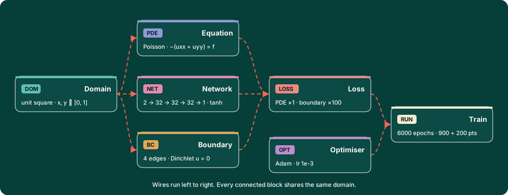
Each ingredient is one block. This is the complete wiring, left to right.
| Block | What it decides | Value for this problem |
|---|---|---|
| DOM Domain | Where the problem lives | Two space dimensions, $x\in[0,1]$, $y\in[0,1]$, no time |
| PDE Equation | What must hold inside | Poisson, $-(u_{xx}+u_{yy}) = f$, with $f = 2\pi^2\sin(\pi x)\sin(\pi y)$ |
| BC Boundary | What is fixed at the edges | $u = 0$ on all four edges (four conditions) |
| NET Network | The family of functions searched | 2 inputs, 3 hidden layers of 32 neurons, $\tanh$, 1 output |
| LOSS Loss | How errors are scored | Mean squared error, weight 1 on the PDE and 100 on the boundary |
| OPT Optimiser | How the weights change | Adam, learning rate $10^{-3}$ |
| RUN Train | How long, and with how many points | 6000 epochs, about 900 interior points and 200 boundary points (50 per edge) |
The wiring rule to remember: the Domain feeds everything that touches space, and the Equation, the Network and the Boundary all feed the Loss. The Loss and Optimiser then feed Train.
A note on labels. The Lab's wording can differ slightly from the names above. Set the quantity and, if a name does not match exactly, pick the nearest field.
4. Step by step in the Lab
Step 1: Domain (DOM)
Add a Domain block. Make it two-dimensional, with $x$ from 0 to 1 and $y$ from 0 to 1. Leave time off.
Check: two coordinates, no time axis.
Step 2: Equation (PDE)
Add an Equation block, connect the Domain to it, and choose Poisson. Enter the source term
$$ f(x,y) = 2\pi^2\sin(\pi x)\sin(\pi y) $$
in the field's syntax (typically 2*pi**2*sin(pi*x)*sin(pi*y)). The equation is $-\nabla^2 u = f$ with a minus sign, so be careful: a flipped sign returns an upside-down solution.
Check: the summary shows the Poisson equation and your $f$.
Step 3: Boundary conditions (BC)
Add a Boundary block, connect the Domain to it, and set a fixed value (Dirichlet) of 0 on each edge:
| Edge | Where | Type | Value |
|---|---|---|---|
| Left | $x = 0$ | Dirichlet | $u = 0$ |
| Right | $x = 1$ | Dirichlet | $u = 0$ |
| Bottom | $y = 0$ | Dirichlet | $u = 0$ |
| Top | $y = 1$ | Dirichlet | $u = 0$ |
Check: the Lab counts four boundary conditions. A square has four edges, and the Lab warns you when the number does not match what the equation needs. If the count is wrong, you have missed an edge.
Step 4: Network (NET)
Add a Network block and connect the Domain to it. Use 2 inputs ($x$ and $y$), 3 hidden layers of 32 neurons, tanh, 1 output ($u$).
Check: the Lab fills in the input size of 2 from the Domain. If you see a size warning, the Network and Domain are not connected, or the input size is not 2.
Step 5: Loss (LOSS)
Add a Loss block. Connect the Equation, the Boundary and the Network to it. Use mean squared error, and set the weights to PDE = 1 and Boundary = 100.
This weighting is the single most important setting in this guide. Section 5 explains why.
Check: the Loss lists two terms, "PDE" and "Boundary".
Step 6: Optimiser (OPT)
Add an Optimiser block: Adam, learning rate 0.001.
Step 7: Train (RUN)
Add the Train block. Connect the Loss and the Optimiser to it. Set 6000 epochs, about 900 interior points (a $30\times30$ grid) and 200 boundary points (50 per edge).
Check: no warnings in the Lab. Remember that a clean check means the configuration is consistent, not that the answer is accurate.
Step 8: Generate and run
Generate the Python code, download the script, and run it on your own computer (pip install torch, then python your_script.py). The Lab builds and checks the configuration, but it does not train the model. A run of this size takes a couple of minutes on a laptop CPU.
Step 9: Judge the result
Do not stop when training finishes. Compare the prediction against the exact solution on a grid that was not used for training.
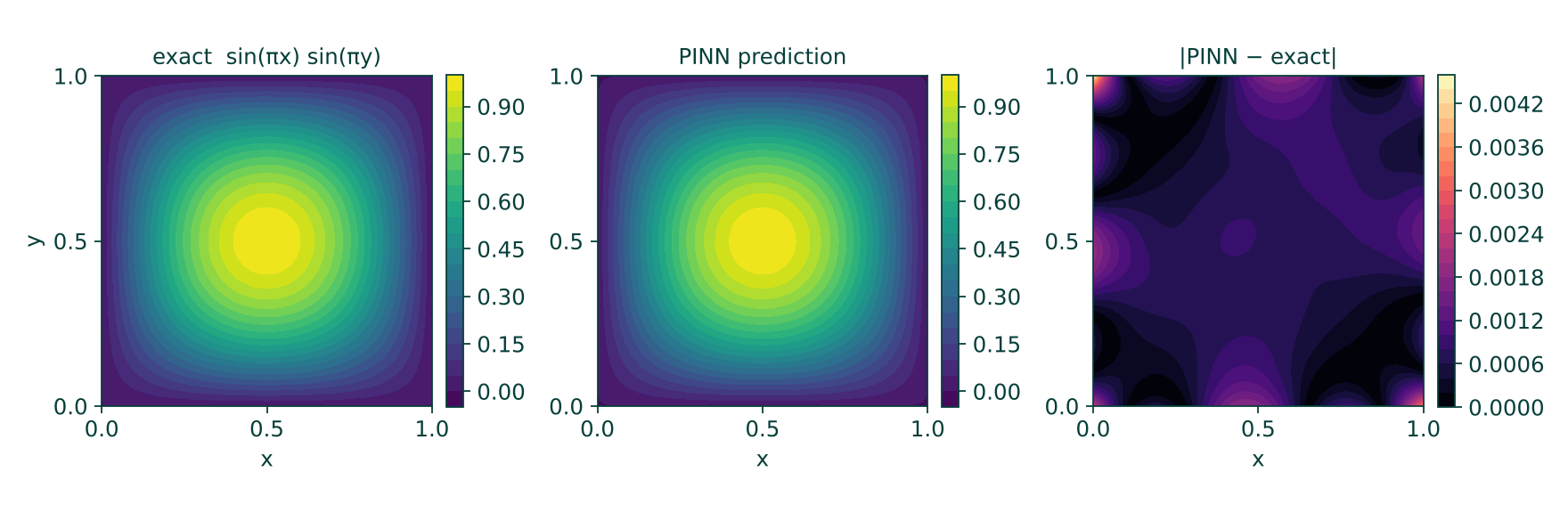
The two surfaces look the same. The third panel is the useful one: it shows where the error lives. In this run it is largest near the edges and corners, and tiny in the middle. That is typical: the boundary is where the network has to match a constraint rather than a smooth interior, and a boundary region with too little weight or too few points is where an error first appears.
The summary number is the relative $L^2$ error,
$$ \varepsilon = \frac{\lVert u_\theta - u_{\text{exact}} \rVert_2}{\lVert u_{\text{exact}} \rVert_2}, $$
evaluated here on a $101\times101$ grid.
What to expect
These figures come from a hand-written reference implementation with exactly the settings above (random seed 0). The Lab's script may start and sample slightly differently, so your numbers will differ, but you should land in the same neighbourhood.
| Epoch | Total loss | Relative $L^2$ error |
|---|---|---|
| 0 | $1 \times 10^{2}$ | $1.1$ |
| 1000 | $5 \times 10^{-2}$ | $1.5 \times 10^{-2}$ |
| 2000 | $5 \times 10^{-3}$ | $2.4 \times 10^{-3}$ |
| 3000 | $3 \times 10^{-3}$ | $1.8 \times 10^{-3}$ |
| 6000 | $1 \times 10^{-3}$ | $1.5 \times 10^{-3}$ |
The largest pointwise error at the end was about $4.5\times10^{-3}$.
Spikes are normal, but keep the best result. In this run the error jumped to about $6\times10^{-2}$ around epochs 4000 and 5000, then fell back by epoch 6000. That is ordinary Adam behaviour on a PINN. A run that ends on a spike is a bad sample of a good method, so keep the best result and not simply the last one.
5. Why the boundary weight matters
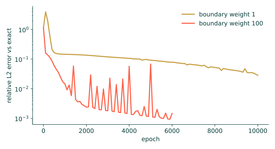
Here is the same problem run twice with everything identical except the boundary weight. With weight 1, the equation term starts around 100 and the boundary term at about 0.015, so the optimiser spends its effort on the equation and the edges are left behind.
| Boundary weight | Epochs | Relative $L^2$ error at the end |
|---|---|---|
| 1 | 10000 | $2.9 \times 10^{-2}$ |
| 100 | 6000 | $1.5 \times 10^{-3}$ |
A weight of 100 reached a better answer in 40% fewer epochs, roughly twenty times more accurate. The reason is that a PINN's equation loss and boundary loss are different quantities with different sizes, and nothing in the method says they should be equal. If the boundary is not being met, raise its weight.
A useful rule. If the loss falls but the error against the exact solution stays high and is worst along the edges, the boundary is under-weighted. Raise the boundary weight by a factor of ten and run again.
6. If something goes wrong
| What you see | Likely cause | What to try |
|---|---|---|
| The error stays near $10^{-1}$ and is worst on the edges | Boundary weight too low | Raise it to 100 (Section 5) |
| The solution is upside down | Sign of the source term | The equation is $-\nabla^2 u = f$ |
| A warning about the number of boundary conditions | An edge is missing | A square needs four conditions |
Loss is nan |
Learning rate too high, or a typo in $f$ | Lower to $10^{-4}$, recheck $f$ |
| A warning about network input size | Network not connected to the 2D Domain | The input size must be 2 |
| Very noisy error curve | Normal for Adam | Judge by where it settles, and keep the best result |
7. Try it yourself
- A different mode. Set $f(x,y)=5\pi^2\sin(2\pi x)\sin(\pi y)$. The exact solution is $u = \sin(2\pi x)\sin(\pi y)$ with the same zero boundaries. Only the Equation block changes. Does the network still reach a similar error?
- Fewer points. Cut the interior points to a $10\times10$ grid. How does the error between the training points change?
- Weights. Try boundary weights of 10 and 1000. Is there a point where raising it further stops helping?
- A smaller network. Try 2 layers of 16 neurons.
8. Next: comparing with the finite element method
A PINN's answer is only worth trusting when it has been checked against something independent. For this problem there are two ways to check: the exact solution above, and a finite element solution on a mesh. The FEM gives a clean benchmark because its error is well understood: for bilinear elements on this problem the error falls in proportion to $h^2$, where $h$ is the element size.
A reference FEM solver, poisson_2d_fem_reference.py, is provided with this guide. It uses bilinear (Q1) elements on a structured mesh and measures the error on the same $101\times101$ grid used for the PINN above, so the two can sit in one table.
| Mesh | Element size $h$ | Relative $L^2$ error | Observed order |
|---|---|---|---|
| $4\times4$ | 0.250 | $6.0\times10^{-2}$ | |
| $8\times8$ | 0.125 | $1.5\times10^{-2}$ | 2.0 |
| $16\times16$ | 0.0625 | $3.8\times10^{-3}$ | 2.0 |
| $32\times32$ | 0.0312 | $9.5\times10^{-4}$ | 2.0 |
| $64\times64$ | 0.0156 | $2.4\times10^{-4}$ | 2.0 |
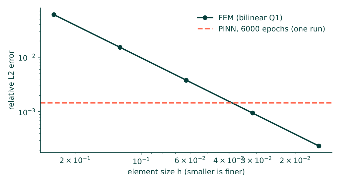
On this one run the PINN's error of about $1.5\times10^{-3}$ sits between the $16\times16$ and $32\times32$ FEM meshes. Read that carefully:
- It is one run. The PINN's error moves around from run to run and during a run. A fair comparison needs several runs with different random seeds, reported as a spread.
- The costs are different. The FEM solved these meshes in a fraction of a second. The PINN took about a minute and a half on a laptop-class CPU. Accuracy per unit of computing time currently favours FEM on a smooth problem like this one.
- The strengths are different. FEM needs a mesh, while a PINN does not. A PINN also gives a continuous function and can fold in measured data. The comparison you build later should weigh those as well as raw error.
When you run the comparison yourself, use the same test grid and the same error measure for both methods, record the training time for the PINN and the solve time for the FEM, and repeat the PINN with several seeds.
9. Recap
- The 2D problem is the same idea as 1D with two inputs, four boundary edges and second derivatives in both directions.
- Wire the Domain into the Equation, Network and Boundary, send those into the Loss, then send the Loss and the Optimiser into Train.
- Weight the boundary. With equal weights the edges are poorly met, and a weight of 100 made the answer about twenty times more accurate.
- Judge a result by where the error is, not just how large it is.
- Compare against an independent reference. The exact solution and FEM give you two.
Reference code for the numbers quoted above: poisson_2d_reference.py (PINN) and poisson_2d_fem_reference.py (FEM). Both are written by hand for checking this guide and are not the Lab's generated output.