Why the weights matter
A network cannot satisfy every term of the loss exactly, so the weights decide the compromise it settles on and the order in which it works. Off by a few orders of magnitude, they decide whether it solves the problem at all.
A PINN loss is a weighted sum of terms, one for the equation and one for each condition (Section 6.1):
$$L(\theta) = w_r\,L_r(\theta) + w_b\,L_b(\theta) + w_0\,L_0(\theta) + \cdots$$
If a network could make every term exactly zero, the weights would not matter: any positive weights give the same minimiser. A network never can. It reaches a compromise, a point where lowering one term would raise another, and the weights decide which compromise. They also decide the order of the work, because the gradient is $w_r\nabla L_r + w_b\nabla L_b + \cdots$ and a term with a large weight dominates the direction of every step. Adam is unaffected by multiplying the whole loss by a constant (Section 3.5), but not by changing the ratio of the weights.
The terms come with their own sizes
The weights are not the only thing that sets the balance. Each term carries the size of its quantity. Take Section 9.1's problem written as the Studio writes it, with nothing divided out:
$$-u'' = (4\pi)^2\sin(4\pi x), \qquad u(0) = u(1) = 0.$$
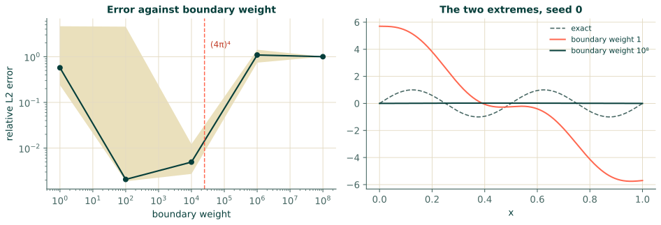
A network that gets the solution's shape wrong by 1% has a residual of about $0.01\times(4\pi)^2$, so the equation term is about $(4\pi)^4 \approx 2.5\times10^4$ times larger than a boundary term for the same 1% mistake. With equal weights, the boundary barely counts. Here is the boundary weight swept over eight orders of magnitude, three seeds each:
import math
import torch
import torch.nn as nn

def d(y, x):
    return torch.autograd.grad(y, x, torch.ones_like(y), create_graph=True)[0]

k = 4 * math.pi
f = lambda x: k**2 * torch.sin(k * x)                    # -u'' = f, unscaled
exact = lambda x: torch.sin(k * x)
x_test = torch.linspace(0, 1, 2001).reshape(-1, 1)

def train(w_b, seed, epochs=5000):
    torch.manual_seed(seed)
    net = nn.Sequential(nn.Linear(1, 32), nn.Tanh(), nn.Linear(32, 32), nn.Tanh(),
                        nn.Linear(32, 32), nn.Tanh(), nn.Linear(32, 1))
    u = lambda x: net(2 * x - 1)
    x = torch.rand(128, 1).requires_grad_(True)
    x_b = torch.tensor([[0.0], [1.0]])
    opt = torch.optim.Adam(net.parameters(), lr=1e-3)
    for epoch in range(epochs):
        opt.zero_grad()
        loss_r = ((-d(d(u(x), x), x) - f(x)) ** 2).mean()        # the equation term
        loss_b = (u(x_b) ** 2).mean()                            # the boundary term
        (loss_r + w_b * loss_b).backward()
        opt.step()
    with torch.no_grad():
        error = ((u(x_test) - exact(x_test)).norm() / exact(x_test).norm()).item()
        return error, u(x_b).abs().max().item()

print("boundary weight    relative L2 error (3 seeds)      largest |u| at the ends")
for w_b in (1, 1e2, 1e4, 1e6, 1e8):
    runs = [train(w_b, seed) for seed in range(3)]
    print(f"{w_b:12.0e}       " + "  ".join(f"{e:.1e}" for e, _ in runs) + "       "
          + "  ".join(f"{b:.0e}" for _, b in runs))
boundary weight    relative L2 error (3 seeds)      largest |u| at the ends
       1e+00       4.6e+00  5.7e-01  2.4e-01       6e+00  7e-01  3e-01
       1e+02       1.9e-03  2.1e-03  4.5e+00       2e-03  2e-04  4e-04
       1e+04       2.7e-03  4.9e-03  1.2e-02       2e-04  7e-04  2e-02
       1e+06       1.4e+00  1.1e+00  7.4e-01       9e-05  1e-02  7e-04
       1e+08       1.0e+00  1.0e+00  1.0e+00       1e-05  4e-07  1e-03
With equal weights the boundary is not met: the networks' values at the ends are between 0.3 and 6, and the errors between 24% and 460%. A boundary weight of $10^2$ or $10^4$ brings five of the six runs down to between $2\times10^{-3}$ and $1.2\times10^{-2}$. At $10^6$ the boundary is met and the errors are back above 70%, and at $10^8$ every run has found $u = 0$: the trivial solution of Section 6.2, which meets the boundary exactly and the equation not at all, an error of exactly 100%. Over eight orders of magnitude of weight the error changes by a factor of a thousand, and the good range is about two orders wide. One run at $10^2$ failed even so, with its boundary met: the weights set the balance, not the outcome of every run.
Two kinds of imbalance
The experiment shows the two ways the balance can fail, and they look different.
- A condition that is too light is not met. The network satisfies the equation with whatever values at the edges are cheapest, one of the family of solutions Section 6.3 met: $\sin(4\pi x)$ plus a smooth correction that the equation cannot see.
- A condition that is too heavy is met at the expense of everything else. Every change to the network that moves its boundary values is now very expensive, the equation is learnt slowly if at all, and at the extreme the cheapest way to meet the boundary, $u = 0$, wins.
Between the two lies a range of good weights, here $10^2$ to $10^4$, and the ratio of the natural sizes of the terms, $(4\pi)^4 \approx 2.5\times10^4$, sits at its upper end. That is not a coincidence, and the next section turns it into a rule.
In the Studio
The Loss block's PDE weight, BC weights (one per BC block) and IC weights (one per IC block) are the $w$ above. The Studio writes the residual exactly as the equation is entered, so these weights are where the sizes of the terms must be balanced, unless the equation itself was scaled first (Section 4.5). The weight of 100 on the boundary in Poisson on a square is an example: its residual's natural size is $2\pi^2 \approx 20$, so the ratio of the squares is about 400.
Exercises
- Show that multiplying every weight by the same constant does not change Adam's steps (ignore Adam's small $\varepsilon$).
- With the residual divided by $(4\pi)^2$, as in Chapter 9, which boundary weight plays the role that $2.5\times10^4$ plays here?
- A heat problem has an initial-condition term and two boundary terms. The initial temperature is of size 300 and the boundary temperatures of size 20. Should the three condition weights be equal?
Answers
- Every gradient is multiplied by the constant $c$, so Adam's running averages become $c\,m$ and $c^2v$, and the step $m/\sqrt{v}$ is unchanged. Only the ratios between the weights reach the optimiser.
- A weight of 1: dividing the residual by $(4\pi)^2$ divides the equation term by $(4\pi)^4$, which is what the weight $2.5\times10^4$ did to the other side of the balance. Chapter 9's runs used exactly this.
- Not if they are to measure relative errors equally: a 1% error costs $3^2 = 9$ in the initial-condition term and $0.2^2 = 0.04$ in a boundary term. Weights of $1/300^2$ and $1/20^2$, or one scale for the whole temperature (Section 10.2), put them on an equal footing.
Recap
- Weights choose the compromise a network settles on and the order in which it attends to the terms; only their ratios matter to Adam.
- Each term carries the size of its quantity. Unscaled, the equation term here was $2.5\times10^4$ times heavier than the boundary term, and equal weights left the boundary unmet.
- Too light a condition is not met; too heavy a condition starves the equation, down to the trivial solution. The good range lies around the ratio of the terms' natural sizes.