Collocation points
The equation is only enforced where you look. How many points, how evenly they are spread, and whether they stay put during training all change the answer.
Section 6.1 showed that the equation term of a PINN loss is an average over collocation points, a Monte Carlo estimate of an integral, and Section 6.5 that a network can satisfy the equation at a few points and badly everywhere else. This section turns those observations into choices: how to spread the points, how many to use, and whether to keep them fixed. Section 3.3 promised a comparison of fixed and freshly drawn points; it is here.
Four ways to spread points
| Strategy | How the points are made | Character |
|---|---|---|
| Regular grid | equally spaced in each direction | perfectly even, but every point lies on a few lines (Section 6.1's aliasing) |
| Uniform random | independent uniform draws | unbiased, but clumps and gaps appear by chance |
| Latin hypercube | each coordinate's range cut into $n$ strips, one point per strip, strips paired at random | even in every single coordinate (McKay et al., 1979) |
| Sobol sequence | a deterministic low-discrepancy sequence, scrambled | even at every scale; quasi-random, not random (Sobol', 1967) |
Figure 7.1 shows 256 points of each kind in the unit square. The random set has visible clumps and holes; the Latin hypercube is even along each axis; the Sobol set is even everywhere, without the grid's lines.
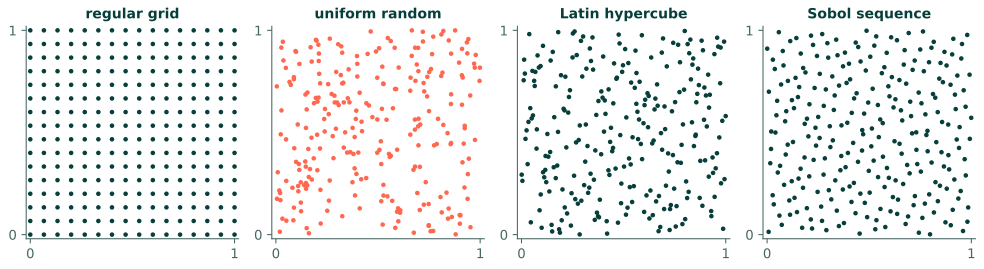
How even a set is shows up directly in how well its average estimates an integral, which is exactly the job the equation term does. Here is the error of the average of $e^{x}\cos y$ over the unit square, against the exact integral $(e - 1)\sin 1$, averaged over 20 draws of each kind. The functions follow the Studio's own sampling code:
import math
import torch

def unit_samples(n, dim, strategy, seed=0):
    """n points in [0, 1]^dim, as the Studio's generated scripts make them."""
    g = torch.Generator().manual_seed(seed)
    if strategy == "sobol":
        return torch.quasirandom.SobolEngine(dimension=dim, scramble=True, seed=seed).draw(n)
    if strategy == "latin hypercube":
        return torch.stack([(torch.randperm(n, generator=g) + torch.rand(n, generator=g)) / n
                            for _ in range(dim)], dim=1)
    return torch.rand(n, dim, generator=g)                              # uniform random

integrand = lambda p: torch.exp(p[:, 0]) * torch.cos(p[:, 1])
exact = (math.e - 1) * math.sin(1)

print("strategy           n = 64     256      1024      4096   (mean error of the average)")
for strategy in ["uniform random", "latin hypercube", "sobol"]:
    row = []
    for n in (64, 256, 1024, 4096):
        errors = [abs(integrand(unit_samples(n, 2, strategy, s).double()).mean().item() - exact) for s in range(20)]
        row.append(sum(errors) / len(errors))
    print(f"{strategy:16s}  " + "  ".join(f"{e:8.1e}" for e in row))
strategy           n = 64     256      1024      4096   (mean error of the average)
uniform random     4.7e-02   2.1e-02   1.3e-02   7.3e-03
latin hypercube    5.4e-03   3.1e-03   1.8e-03   8.8e-04
sobol              1.1e-03   7.4e-05   9.4e-06   5.4e-07
Uniform random points improve like $1/\sqrt{n}$: four times the points, half the error. The Latin hypercube starts about ten times better on this smooth integrand and improves at a similar rate. The Sobol set improves faster still, by a factor of about two thousand for sixty-four times the points, and at 4096 points it is four orders of magnitude ahead of plain random points. For a smooth residual, a Sobol set of $n$ points measures the equation about as well as a random set of very many more.
Fixed points or fresh ones
There is a second choice, independent of the first: draw the collocation points once and keep them, or draw new ones during training. Fresh points mean the network can never fit a particular finite set, because the set keeps changing; the price is a noisier loss, exactly like the mini-batch gradients of Section 3.3.
The test problem is Section 6.5's, $-u'' = (4\pi)^2\sin(4\pi x)$ with zero ends, three seeds per setting, uniform random points, either drawn once or redrawn at every epoch:
import torch.nn as nn

def d(y, x):
    return torch.autograd.grad(y, x, torch.ones_like(y), create_graph=True)[0]

k = 4 * math.pi
f = lambda x: k**2 * torch.sin(k * x)
residual = lambda u, x: -d(d(u(x), x), x) - f(x)
x_test = torch.linspace(0, 1, 2001).reshape(-1, 1)

def train(n_col, resample, seed=0, epochs=4000):
    torch.manual_seed(seed)
    net = nn.Sequential(nn.Linear(1, 32), nn.Tanh(), nn.Linear(32, 32), nn.Tanh(),
                        nn.Linear(32, 32), nn.Tanh(), nn.Linear(32, 1))
    u = lambda x: net(2 * x - 1)
    x_col = torch.rand(n_col, 1).requires_grad_(True)
    x_b = torch.tensor([[0.0], [1.0]])
    opt = torch.optim.Adam(net.parameters(), lr=1e-3)
    for epoch in range(epochs):
        if resample:
            x_col = torch.rand(n_col, 1).requires_grad_(True)       # fresh points every epoch
        opt.zero_grad()
        loss = (residual(u, x_col) ** 2).mean() / k**4 + (u(x_b) ** 2).sum()
        loss.backward()
        opt.step()
    with torch.no_grad():
        exact = torch.sin(k * x_test)
        return ((u(x_test) - exact).norm() / exact.norm()).item()

print("points   fixed: median (three runs)      redrawn every epoch: median (three runs)")
for n in (8, 32, 128):
    fixed = sorted(train(n, False, s) for s in range(3))
    fresh = sorted(train(n, True, s) for s in range(3))
    print(f"{n:5d}    {fixed[1]:.1e} ({fixed[0]:.0e} to {fixed[2]:.0e})        {fresh[1]:.1e} ({fresh[0]:.0e} to {fresh[2]:.0e})")
points   fixed: median (three runs)      redrawn every epoch: median (three runs)
    8    4.2e+00 (2e+00 to 1e+01)        7.0e-02 (1e-02 to 1e-01)
   32    9.6e-02 (7e-02 to 2e-01)        4.0e-02 (6e-03 to 9e-02)
  128    1.7e-02 (9e-03 to 9e-02)        3.3e-02 (1e-02 to 8e-02)
With 8 fixed points every run fails completely, as in Section 6.5. Redrawing 8 points at every epoch brings the median error down to 7%: over 4000 epochs the network has been checked at 32,000 different places. With 128 points the advantage disappears, and the fixed set is, if anything, slightly better: once the points are dense enough to see every feature of the solution, the noise of redrawing costs more than it gains, as mini-batch noise did near the optimum in Section 3.3.
Rules of thumb
- Use enough points to resolve the solution's finest feature several times over: here, a few points per half-wave was too few to fix and enough to redraw.
- Prefer a Sobol or Latin hypercube set to plain random points when the points are fixed; prefer redrawing when the points are few or the solution is not yet well resolved.
- If you redraw, expect a noisier loss curve, and let the learning rate decay at the end (Section 3.6).
How many points
There is no formula, but there is a check. Train with $N$ points; evaluate the residual at many fresh points (Section 6.5); if it is much larger there than at the training points, $N$ is too small, or the points should be redrawn. Problems with sharp features need points concentrated where the features are, which uniform spreading wastes; that is the next section.
In the Studio
The Domain block sets the count (Interior points) and the spread (Interior distribution: Uniform random,
Regular grid, Latin hypercube or Sobol sequence). The Train block's Resample points every redraws the
interior points every so many epochs; 0, the default, keeps one set for the whole run. Two details of the
generated script are worth knowing: the boundary points are drawn afresh every time a boundary term is computed,
so they are always resampled; and a Sobol set drawn with the same seed is the same set, so "resampling" a Sobol
set changes nothing unless the seed changes
(Read the script).
Exercises
- Why does a Latin hypercube help so much more for $e^x\cos y$ than for a function such as $\sin(8\pi x)\sin(8\pi y)$?
- With 8 points redrawn every epoch for 4000 epochs, how many distinct points has the network been trained on? Why is that not the same as training on 32,000 fixed points?
- A colleague trains with 50,000 fixed points and finds the residual at fresh points equal to the training residual. Should they switch to resampling?
Answers
- A Latin hypercube makes each coordinate's values perfectly even, which is enough for functions that are close to a sum of one-variable pieces; $e^x\cos y$ varies smoothly along each axis. A product of fast oscillations in both directions depends on how the coordinates are paired, which the random pairing does nothing to even out.
- 32,000 (with probability one, all different). But at any one step the loss sees only 8 of them, so each step follows a noisy estimate of the full loss (Section 3.3); 32,000 fixed points give the full, smooth loss at every step, at 4000 times the cost per step.
- No. Equal residuals at training and fresh points mean the fixed set is already dense enough to stand for the whole domain. Resampling would add noise without adding information.
Recap
- Collocation points estimate an integral of the squared residual. Even sets (Latin hypercube, Sobol) estimate it far better than random ones of the same size; a regular grid is even but can be fooled.
- Redrawing points during training stops the network from fitting a particular set: decisive when points are few, unnecessary (and slightly noisy) when they are plentiful.
- Judge the number of points by comparing the residual at fresh points with the residual at the training points.
References
- McKay, M. D., Beckman, R. J., & Conover, W. J. (1979). A comparison of three methods for selecting values of input variables in the analysis of output from a computer code. Technometrics, 21(2), 239–245. doi:10.1080/00401706.1979.10489755
- Sobol', I. M. (1967). On the distribution of points in a cube and the approximate evaluation of integrals. USSR Computational Mathematics and Mathematical Physics, 7(4), 86–112. doi:10.1016/0041-5553(67)90144-9