Curved and awkward domains

The Studio offers three shapes: a line, a rectangle and a disc. Real problems come in others: a plate with a hole, an L-shaped bracket, a channel with a step. A PINN asks nothing of the shape except points, interior points spread evenly and boundary points with their outward normals. There is no mesh to generate, which is a real advantage over mesh-based methods for complicated shapes. It comes with three traps, one for each part of this section.

Even points on a disc

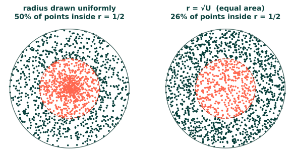
Polar coordinates make it tempting to draw the radius and the angle uniformly. That puts as many points in the inner half of the radius as in the outer half, although the inner disc has only a quarter of the area. The fix is to draw the radius as $r = R\sqrt{U}$, with $U$ uniform on $[0, 1]$: the area within radius $r$ grows like $r^2$, so the square root makes equal areas equally likely. The alternative that works for any shape is rejection sampling: draw points in a box around the shape and keep the ones inside.

import math
import torch

g = torch.Generator().manual_seed(0)
n = 100_000
U = torch.rand(n, 2, generator=g)
naive_r = U[:, 0]                                    # radius drawn uniformly: wrong
equal_area_r = U[:, 0].sqrt()                        # r = sqrt(U): right
box = 2 * torch.rand(n, 2, generator=g) - 1          # rejection: the square around the disc...
kept = box[box.norm(dim=1) < 1]                      # ...keeping what falls inside

def report(name, r):
    inner = (r < 0.5).float().mean().item()
    integral = math.pi * (r**2).mean().item()        # area times the average of r^2
    print(f"{name:12s}  {inner:5.1%} of points within half the radius;  integral of r^2 {integral:.3f}")

print("exact:        25.0% (the inner disc's share of the area);     integral of r^2 1.571")
report("naive polar", naive_r)
report("equal-area", equal_area_r)
report("rejection", kept.norm(dim=1))
print(f"rejection kept {len(kept) / n:.1%} of the candidates (pi/4 = {math.pi / 4:.1%})")

exact:        25.0% (the inner disc's share of the area);     integral of r^2 1.571
naive polar   50.0% of points within half the radius;  integral of r^2 1.047
equal-area    24.9% of points within half the radius;  integral of r^2 1.571
rejection     25.3% of points within half the radius;  integral of r^2 1.567
rejection kept 78.5% of the candidates (pi/4 = 78.5%)

The naive points estimate the integral of $r^2$ over the disc as $\pi/3$ instead of $\pi/2$, a third too small, because they over-represent the middle (Figure 7.3). In the language of Section 7.2, they are drawn from a density proportional to $1/r$: a PINN trained on them minimises a loss that weighs the centre heavily and the rim lightly, a weighting nobody chose. The Studio's Circle geometry uses the equal-area map, so its points are even.

Rejection sampling wastes the candidates that fall outside: about a fifth for a disc in its square, more for thin shapes, and much more in three dimensions, where a ball fills only 52% of its cube. It is still cheap, since candidates cost almost nothing next to training.

Boundary points and their normals

A boundary made of straight edges is handled in two steps: choose an edge with probability proportional to its length, then a point uniformly along it. If the vertices are listed anticlockwise, the domain lies to the left of every edge, so the outward normal is the edge's direction turned a quarter turn clockwise. Two checks from the divergence theorem catch the usual mistakes, a normal pointing inwards or edges sampled unevenly: the outward normals add up to zero round any closed boundary, $\oint \mathbf{n}\,ds = \mathbf{0}$, and since the divergence of $\mathbf{x} = (x, y)$ is 2, $\tfrac12\oint \mathbf{x}\cdot\mathbf{n}\,ds$ is the area. For an L-shaped domain, the square $(-1, 1)^2$ without its lower-right quarter:

def polygon_boundary(vertices, n, generator=None):
    """n points spread evenly along a closed polygon, with outward unit normals.
    The vertices must be listed anticlockwise."""
    P, Q = vertices, vertices.roll(-1, dims=0)                    # edge i runs from P[i] to Q[i]
    length = (Q - P).norm(dim=1)
    edge = torch.multinomial(length / length.sum(), n, replacement=True, generator=generator)
    t = torch.rand(n, 1, generator=generator)
    points = P[edge] + t * (Q[edge] - P[edge])
    tangent = (Q[edge] - P[edge]) / length[edge, None]
    normals = torch.stack([tangent[:, 1], -tangent[:, 0]], dim=1)  # turned clockwise: outward
    return points, normals

L_shape = torch.tensor([[0., 0.], [1., 0.], [1., 1.], [-1., 1.], [-1., -1.], [0., -1.]])
pts, normals = polygon_boundary(L_shape, 100_000, g)
perimeter = (L_shape.roll(-1, dims=0) - L_shape).norm(dim=1).sum().item()
print(f"perimeter {perimeter:.0f};  area from boundary points {0.5 * perimeter * (pts * normals).sum(dim=1).mean().item():.3f} (exact 3)")
print("sum of outward normals:", [round(v, 3) for v in (perimeter * normals.mean(dim=0)).tolist()], "(exact [0, 0])")

perimeter 8;  area from boundary points 3.000 (exact 3)
sum of outward normals: [-0.002, -0.022] (exact [0, 0])

Both checks pass, to within the noise of 100,000 random points. Curved boundaries work the same way: a circle of radius $R$ has outward normal $(x, y)/R$; a boundary given as the zero set of a function $\phi$, negative inside, has outward normal $\nabla\phi/|\nabla\phi|$. A hole is a second boundary whose normals point into the hole, which is out of the domain; list its vertices clockwise and the same function gets them right.

Corners

The L-shape has a re-entrant corner at the origin, where the boundary turns inwards and the interior angle is $3\pi/2$. Corners like this change the solution itself. In polar coordinates the functions $r^\lambda\sin(\lambda\theta)$ satisfy Laplace's equation for any $\lambda$ (they are the imaginary part of $z^\lambda$). Measuring $\theta$ from one edge of the corner, vanishing on both edges, $\theta = 0$ and $\theta = \omega$, requires $\lambda\omega$ to be a multiple of $\pi$. For $\omega = 3\pi/2$ the smallest choice is $\lambda = 2/3$, so near the corner a solution that vanishes on both edges behaves like

$$u \approx c\, r^{2/3}\sin\!\left(\tfrac{2}{3}\theta\right),$$

with $c$ set by the rest of the problem. This is continuous, but its gradient, of size $r^{-1/3}$, is infinite at the corner. A network of tanh neurons is smooth everywhere and cannot have an infinite gradient anywhere; near the corner it can only approximate.

The test problem takes Laplace's equation on the L-shape with the solution $u = r^{2/3}\sin(2\theta/3) + e^x\sin y$, both parts harmonic, and its values imposed on the whole boundary. Three versions are trained with the same network, optimiser and 3000 epochs:

• plain: 2000 interior points spread evenly by rejection;
• points at the corner: the same, with a quarter of the points moved to within 0.2 of the corner, as Section 7.2 would suggest;
• enriched: the trial function $u_\theta = c\,r^{2/3}\sin(2\theta/3) + N_\theta(x, y)$, with the number $c$ learnt along with the weights. The corner's form comes from the geometry; its strength is left to the training.

import torch.nn as nn

def d(y, x):
    return torch.autograd.grad(y, x, torch.ones_like(y), create_graph=True)[0]

def inside(p):                                       # (-1, 1)^2 without the quarter x >= 0, y <= 0
    return (p.abs().max(dim=1).values < 1) & ~((p[:, 0] >= 0) & (p[:, 1] <= 0))

def sample_inside(n, generator):                     # rejection sampling
    pts = torch.empty(0, 2)
    while len(pts) < n:
        candidates = 2 * torch.rand(2 * n, 2, generator=generator) - 1
        pts = torch.cat([pts, candidates[inside(candidates)]])
    return pts[:n]

def corner(p):                                       # r^(2/3) sin(2 theta / 3), theta from the edge y = 0, x > 0
    r = p.norm(dim=1, keepdim=True)
    theta = torch.remainder(torch.atan2(p[:, 1:2], p[:, 0:1]), 2 * math.pi)
    return r ** (2 / 3) * torch.sin(2 * theta / 3)

exact = lambda p: corner(p) + torch.exp(p[:, 0:1]) * torch.sin(p[:, 1:2])

def train_L(variant, epochs=3000, seed=0):
    g = torch.Generator().manual_seed(100 + seed)
    torch.manual_seed(seed)
    net = nn.Sequential(nn.Linear(2, 32), nn.Tanh(), nn.Linear(32, 32), nn.Tanh(),
                        nn.Linear(32, 32), nn.Tanh(), nn.Linear(32, 1))
    c = torch.zeros(1, requires_grad=True)           # the corner's strength (used by "enriched" only)
    if variant == "enriched":
        u = lambda p: c * corner(p) + net(p)
    else:
        u = lambda p: net(p)
    x_in = sample_inside(2000, g)
    if variant == "points at the corner":            # replace a quarter with points within 0.2 of the corner
        near = sample_inside(20000, g)
        x_in = torch.cat([x_in[:1500], near[near.norm(dim=1) < 0.2][:500]])
    x_in.requires_grad_(True)
    x_bd, _ = polygon_boundary(L_shape, 400, g)
    u_bd = exact(x_bd)
    opt = torch.optim.Adam([{"params": net.parameters()}, {"params": [c], "lr": 1e-2}], lr=1e-3)
    for epoch in range(epochs):
        opt.zero_grad()
        grad_u = d(u(x_in), x_in)
        laplacian = d(grad_u[:, 0:1], x_in)[:, 0:1] + d(grad_u[:, 1:2], x_in)[:, 1:2]
        loss = (laplacian ** 2).mean() + ((u(x_bd) - u_bd) ** 2).mean()
        loss.backward()
        opt.step()
    return u, c

xs = torch.linspace(-1, 1, 201)
X, Y = torch.meshgrid(xs, xs, indexing="xy")
grid = torch.stack([X.flatten(), Y.flatten()], dim=1)
grid = grid[~((grid[:, 0] > 0) & (grid[:, 1] < 0))]   # the L-shape, edges included
r = grid.norm(dim=1)
for variant in ["plain", "points at the corner", "enriched"]:
    u, c = train_L(variant)
    with torch.no_grad():
        err = (u(grid) - exact(grid)).abs().flatten()
        rel = ((u(grid) - exact(grid)).norm() / exact(grid).norm()).item()
    print(f"{variant:21s} relative L2 {rel:.1e}   largest error: {err[r < 0.1].max():.1e} near the corner, "
          f"{err[r >= 0.1].max():.1e} elsewhere" + (f"   c = {c.item():.3f}" if variant == "enriched" else ""))

plain                 relative L2 3.0e-02   largest error: 2.3e-01 near the corner, 1.6e-01 elsewhere
points at the corner  relative L2 3.0e-02   largest error: 2.3e-01 near the corner, 1.6e-01 elsewhere
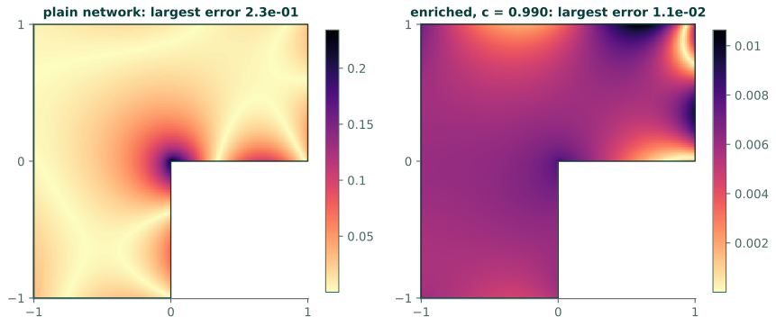
enriched              relative L2 5.5e-03   largest error: 8.1e-03 near the corner, 1.1e-02 elsewhere   c = 0.990

The plain network's error is 3%, largest at the corner, and not only there: away from the corner the largest error is still 0.16, most of the size of the error at the corner itself (Figure 7.4). Moving a quarter of the points to the corner changed nothing, to two digits. This is the difference between a sampling problem, which Section 7.2's methods address, and a representation problem: more points ask more insistently for a function the network cannot produce. The enriched version learnt $c = 0.990$, close to the exact value of 1. Its error is five times smaller overall and about thirty times smaller at the corner, which is no longer where the error is largest.

When the form of a singularity is known, from the geometry (corners, cracks) or from the physics (a point load, a point source), build it into the trial function, as Section 6.4 built in conditions, and leave its strength to the training. Finite-element analysis treats crack tips the same way, with special functions that carry the singular behaviour.

Building conditions into awkward shapes

Section 6.4's trial function $u = G + D\,N$ needs a function $D$ that is zero on the boundary and only there. For a disc, $D = 1 - (x^2 + y^2)/R^2$ does it. For a polygon, the obvious choice, the product of the distances to each edge's line, fails as soon as the shape is not convex: for the L-shape, the line through the edge $y = 0$, $x > 0$ carries on through the domain at $x < 0$, so $D$ would vanish on a line inside the domain and pin the solution to zero there. Sukumar & Srivastava (2022) show how to combine the edges' distance functions so that the result vanishes on the boundary alone, for polygons and curved shapes, and how to impose Neumann and Robin conditions the same way.

In the Studio

The Domain block's geometries are Line, Rectangle and Circle, and a circle is sampled with the equal-area map. Any other shape is an edit to the generated script, in two places. Replace sample_interior with a rejection sampler like sample_inside above, and make each boundary function, sample_bc1 to sample_bc4 on a rectangle, return its piece of the boundary as a pair of points and outward normals, as polygon_boundary does. Keep the shape inside the rectangle set in the Domain block, because the script scales the network's inputs with that rectangle. The L-shape fits this pattern well: its six edges face only four directions, so the rectangle's four boundary terms can carry them, with the inner corner's two edges joining the right and bottom groups whose normals they share.

Exercises

1. Draw points evenly in the ring between radii 1 and 2. What should replace $r = \sqrt{U}$?
2. A crack is a corner with interior angle $2\pi$. What does the argument above give for the behaviour near its tip? And for the convex corner of a square, angle $\pi/2$?
3. The enriched run gave its coefficient its own learning rate of $10^{-2}$. Why would $10^{-3}$, the network's rate, have been a poor choice for it?

Recap

• A PINN needs points, not a mesh. Spread them by area: $r = R\sqrt{U}$ on a disc, rejection sampling for any shape with an inside test.
• Boundary points need outward normals. For a polygon listed anticlockwise, turn each edge clockwise; check that the normals sum to zero and that $\tfrac12\oint\mathbf{x}\cdot\mathbf{n}\,ds$ gives the area.
• Re-entrant corners make the solution singular, which a smooth network cannot represent and more points cannot fix. When the form of a singularity is known, build it into the trial function.

References

- Sukumar, N., & Srivastava, A. (2022). Exact imposition of boundary conditions with distance functions in physics-informed deep neural networks. Computer Methods in Applied Mechanics and Engineering, 389, 114333. doi:10.1016/j.cma.2021.114333