Manufactured solutions: invent the answer, then build the problem
A way to test any PINN on a problem with no textbook solution. Choose the answer first, let a computer algebra system work out the source term and the boundary data, and use a mixed Dirichlet and Neumann boundary.
So far every problem came with a tidy exact answer, found by guessing a sine and checking. Real problems do not. This guide teaches the trick that lets you test a PINN on almost any equation anyway: the method of manufactured solutions.
The idea is simple and slightly backwards. Instead of starting from a problem and hunting for its solution, you invent the solution first and then work out which problem it solves. You then hand that problem to the Studio and check that the network finds your invented answer.
Before you start. Finish the two Poisson guides first, including Poisson on a square. Open the Studio and choose an empty canvas.
1. The method in four steps
- Choose a solution. Write any smooth function $u^\ast(x,y)$ that is rich enough to use every term of the equation. It does not need to mean anything physically.
- Differentiate it to find the source term $f$ that makes the equation true.
- Evaluate it on the boundary to find the boundary data. If a boundary condition involves a derivative, differentiate first, then evaluate.
- Solve the problem you have now defined, and compare with $u^\ast$.
Because the answer is known by construction, the comparison in step 4 is an honest test of the whole pipeline: the equation entered, the boundary conditions entered, the network, the loss, and the optimiser.
Why this is worth the trouble. If a PINN fails on a real problem you cannot tell whether the method failed or you made a typing mistake in the equation. A problem with a known answer separates the two. Run a manufactured version first, get it right, then change to the real data.
2. The problem we will manufacture
Take the unit square $\Omega = (0,1)\times(0,1)$ and choose
$$ u^\ast(x,y) = e^{x}\sin(\pi y) + x\,y . $$
It has an exponential in one direction, a sine in the other, and a cross term, so it is not symmetric and not a product of simple pieces.
Step 1: the source term
The Studio writes Poisson's equation as
$$ \nabla^2 u = f \qquad \Bigl(\text{that is } \tfrac{\partial^2 u}{\partial x^2}+\tfrac{\partial^2 u}{\partial y^2} = f\Bigr), $$
with no minus sign. (If your textbook writes $-\nabla^2 u = g$, the Studio's $f$ is $-g$. A flipped sign is the classic manufactured-solution mistake: the network returns the right shape, upside down.)
Differentiating $u^\ast$:
$$ \frac{\partial^2 u^\ast}{\partial x^2} = e^{x}\sin(\pi y), \qquad \frac{\partial^2 u^\ast}{\partial y^2} = -\pi^2 e^{x}\sin(\pi y), $$
and the cross term $xy$ has zero Laplacian. So
$$ f(x,y) = \nabla^2 u^\ast = (1-\pi^2)\,e^{x}\sin(\pi y). $$
You do not have to do this by hand. Here is the whole of step 2 and step 3 in a few lines of SymPy:
import sympy as sp
x, y = sp.symbols("x y")
u = sp.exp(x) * sp.sin(sp.pi * y) + x * y

f = sp.simplify(sp.diff(u, x, 2) + sp.diff(u, y, 2))   # source term
print(f)                                  # (1 - pi**2)*exp(x)*sin(pi*y)
print(u.subs(x, 0), u.subs(y, 0), u.subs(y, 1))        # edge values
print(sp.diff(u, x).subs(x, 1))           # normal derivative on x = 1
Using a computer algebra system for this step is the point: by hand it is easy to drop a sign or a factor.
Step 2: the boundary data, with a mix of conditions
Now we make the boundary interesting. Three edges get a Dirichlet condition (the value of $u$ is given) and one edge gets a Neumann condition (the slope across the edge is given). Neumann conditions say how fast the solution is leaving through an edge: physically, a heat flux.
| Edge | Where | Condition | Data from $u^\ast$ |
|---|---|---|---|
| Left | $x = 0$ | Dirichlet | $u = \sin(\pi y)$ |
| Bottom | $y = 0$ | Dirichlet | $u = 0$ |
| Top | $y = 1$ | Dirichlet | $u = x$ |
| Right | $x = 1$ | Neumann | $\dfrac{\partial u}{\partial x} = e\,\sin(\pi y) + y$ |
Where the numbers come from:
- Left: $u^\ast(0,y) = e^0\sin(\pi y) + 0 = \sin(\pi y)$.
- Bottom: $u^\ast(x,0) = e^{x}\cdot 0 + 0 = 0$.
- Top: $u^\ast(x,1) = e^{x}\sin\pi + x = x$, because $\sin\pi = 0$.
- Right: first differentiate, $\partial u^\ast/\partial x = e^{x}\sin(\pi y) + y$, then put $x = 1$. The outward normal on the right edge points in the $+x$ direction, so the normal derivative is exactly $\partial u/\partial x$ there.
Differentiate first, then evaluate. Substituting $x=1$ into $u^\ast$ before differentiating gives a function with no $x$ left in it, and its derivative with respect to $x$ is zero. That is wrong. The boundary value of a derivative is not the derivative of the boundary value.
The problem is well posed: a Dirichlet condition on at least one edge pins down the solution uniquely.
3. How a PINN sees the problem
Everything from the 2D guide carries over: a network $u_\theta(x,y)$ and a residual,
$$ r_\theta(x,y) = \frac{\partial^2 u_\theta}{\partial x^2} + \frac{\partial^2 u_\theta}{\partial y^2} - f(x,y). $$
The new part is the Neumann edge. A Dirichlet condition compares the network's value with data; a Neumann condition compares its derivative with data, so it needs automatic differentiation too:
$$ \mathcal{L}(\theta) = \underbrace{\overline{r_\theta^{\,2}}}_{\text{PDE}} + w_{\text{D}}\Bigl[\,\overline{(u_\theta - g_{\text{left}})^2} + \overline{(u_\theta - g_{\text{bottom}})^2} + \overline{(u_\theta - g_{\text{top}})^2}\,\Bigr] + w_{\text{N}}\,\overline{\Bigl(\tfrac{\partial u_\theta}{\partial x} - h_{\text{right}}\Bigr)^2}, $$
where the bar means the average over that edge's sample points.
4. The plan: one block per decision
| # | Block | The question it answers | Our choice |
|---|---|---|---|
| 1 | DOM Domain | Where does the problem live? | Two space dimensions, $x,y\in[0,1]$, no time |
| 2 | PDE Equation | Which equation must hold inside? | Poisson, $\nabla^2 u = f$, with $f = (1-\pi^2)\,e^{x}\sin(\pi y)$ |
| 3 | BC Boundary | What is fixed at the edges? | Three Dirichlet edges, one Neumann edge (table above) |
| 4 | NET Network | What function family do we search in? | 2 inputs, 3 hidden layers of 32 neurons, $\tanh$, 1 output |
| 5 | LOSS Loss | How do we score the errors? | Mean squared error, weight 1 on the PDE and 100 on every boundary term |
| 6 | OPT Optimiser | How do the weights change? | Adam, learning rate $10^{-3}$ |
| 7 | RUN Train | How long and with how many points? | 6000 epochs, about 900 interior points, 50 points per edge |
A note on labels. The Studio's wording can differ slightly between versions. The quantity to set is what matters; if a field name does not match this page exactly, pick the nearest one. If a value is not offered, keep the Studio's default.
5. Step by step in the Studio
Step 1: Domain (DOM)
Add a Domain block. Make it two-dimensional, $x$ from 0 to 1 and $y$ from 0 to 1, with time off.
Step 2: Equation (PDE)
Add an Equation block, connect the Domain, and choose Poisson. Enter the source term in the field's syntax:
(1 - pi**2) * exp(x) * sin(pi*y)
Check: the summary reads $\nabla^2 u = f$ with this $f$, and no minus sign in front of the Laplacian. This is the line where the sign mistake happens, so read it twice.
Step 3: Boundary conditions (BC)
Add a Boundary block, connect the Domain to it, and add four conditions:
| Edge | Type | Value to enter |
|---|---|---|
| Left, $x=0$ | Fixed value (Dirichlet) | sin(pi*y) |
| Bottom, $y=0$ | Fixed value (Dirichlet) | 0 |
| Top, $y=1$ | Fixed value (Dirichlet) | x |
| Right, $x=1$ | Neumann (normal derivative) | exp(1)*sin(pi*y) + y |
Notice that two of the Dirichlet values are expressions in the coordinate along the edge, not just constants. Use exp(1) for $e$.
Check: the Studio counts four conditions, one per edge.
Step 4: Network (NET)
Add a Network block, connect the Domain to it, and use 2 inputs, 3 hidden layers of 32 neurons, tanh, and 1 output.
Step 5: Loss (LOSS)
Add a Loss block, connect the Equation, Boundary and Network to it, use mean squared error, and set the weights to PDE = 1 and boundary = 100 for every condition. If the Studio asks for the boundary weights as a list, one per condition in the order above, enter [100, 100, 100, 100].
Step 6: Optimiser and Train
Add an Optimiser block (Adam, learning rate 0.001) and a Train block (6000 epochs, about 900 interior points, 50 points per edge). Connect the Loss and Optimiser to Train.
Check: no warnings. As always, a clean check means consistent, not accurate.
Step 7: Generate and run
Generate the Python code, download the script and run it on your own computer. The Studio builds and checks the configuration; training happens in your script. A run of this size takes a couple of minutes on a laptop CPU.
Step 8: Judge the result
Compare with $u^\ast$ on a $101\times101$ grid that was not used for training.
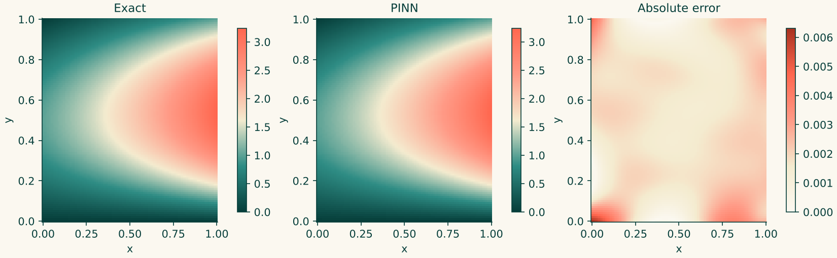
The two surfaces agree, and the error panel again shows where the work is hard. In the reference run the largest error, about $6\times10^{-3}$, sat in the bottom-left corner, where two Dirichlet edges meet. The Neumann edge on the right was not the worst place: its largest error was about $3\times10^{-3}$, about the same as the largest error in the interior.
The summary number is the relative $L^2$ error against $u^\ast$,
$$ \varepsilon = \frac{\lVert u_\theta - u^\ast \rVert_2}{\lVert u^\ast \rVert_2}. $$
What to expect
These figures come from a hand-written reference implementation with exactly the settings above (random seed 0). The Studio's script may initialise and sample slightly differently, so your numbers will differ, but you should land in the same neighbourhood.
| Epoch | Total loss | Relative $L^2$ error |
|---|---|---|
| 0 | $1 \times 10^{3}$ | $1.2$ |
| 1000 | $9 \times 10^{-1}$ | $5.9 \times 10^{-3}$ |
| 2000 | $8 \times 10^{-2}$ | $1.5 \times 10^{-3}$ |
| 3000 | $3 \times 10^{-2}$ | $9.4 \times 10^{-4}$ |
| 6000 | $7 \times 10^{-3}$ | $1.2 \times 10^{-3}$ |
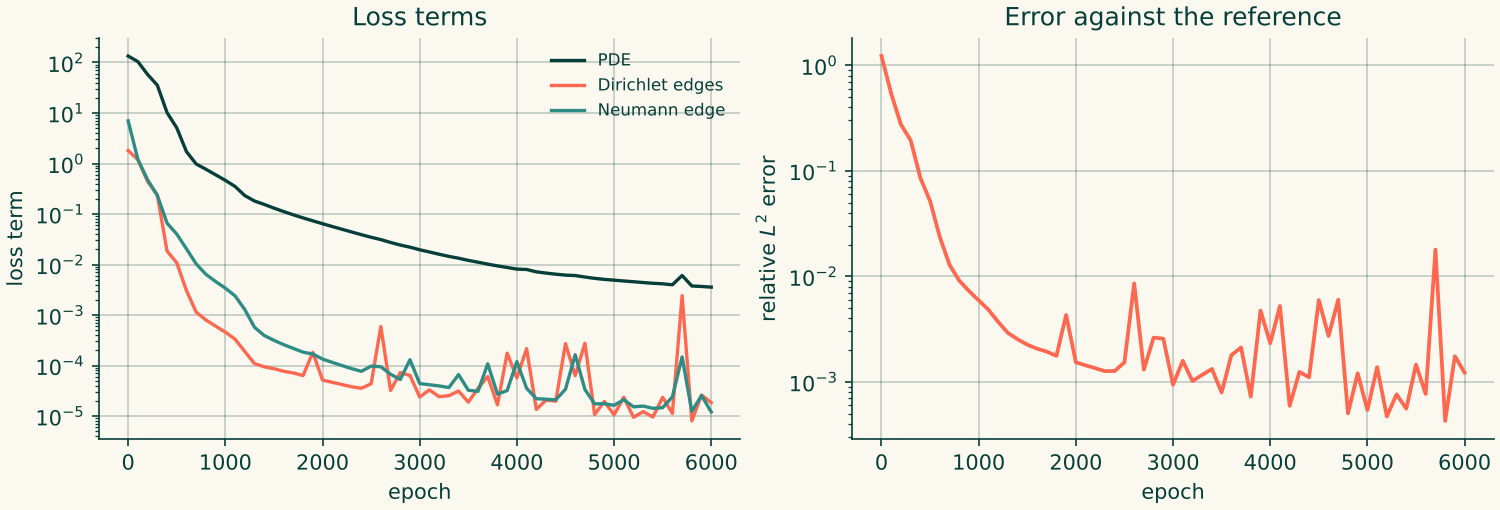
The loss curves are worth reading. The Dirichlet and Neumann terms fall very quickly because they are heavily weighted, and the PDE term is the one that takes thousands of epochs.
Keep the best result. During the last third of training the error spiked once to about $2\times10^{-2}$ and otherwise wobbled around $10^{-3}$, and the best value in the run ($4\times10^{-4}$, near epoch 5800) did not land on the last epoch. That is normal for Adam. Save the best, not simply the last.
6. Does the boundary weight matter here?
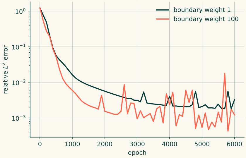
Same problem, with the boundary weight dropped from 100 to 1.
| Boundary weight | Error at epoch 1000 | Median error, epochs 4000 to 6000 | Error at epoch 6000 | Largest pointwise error at epoch 6000 |
|---|---|---|---|---|
| 1 | $1.6 \times 10^{-2}$ | $2.1 \times 10^{-3}$ | $3.2 \times 10^{-3}$ | $1.3 \times 10^{-2}$, on the Neumann edge |
| 100 | $5.9 \times 10^{-3}$ | $1.2 \times 10^{-3}$ | $1.2 \times 10^{-3}$ | $6.3 \times 10^{-3}$, in a corner |
A weight of 100 was clearly faster early on (about three times lower error at epoch 1000) and about 1.7 times better in the median over the last third of training. That is a much smaller gap than in the unit-square Poisson guide, and these are single runs with one seed, so treat it as a tendency and not a law. Note also that the weight-100 curve is much noisier, with spikes up and down, while the weight-1 curve is smooth: single-epoch values, such as the final one, can mislead in either direction, which is why the table includes a median.
What is more telling is where the large error went. With weight 1 the biggest error sat on the Neumann edge, which is consistent with a slope condition being the easiest constraint to neglect when the equation term dominates the loss. If you ever see a boundary that is not being honoured, raise its weight first.
7. If something goes wrong
| What you see | Likely cause | What to try |
|---|---|---|
| The solution is the right shape but upside down or the wrong size | Sign convention in $f$. The Studio uses $\nabla^2 u = f$ | Enter $f=\nabla^2u^\ast$ as above, not $-\nabla^2u^\ast$ |
| The error is large only on the Neumann edge | Neumann data wrong (substituted before differentiating) or its weight too low | Recompute $\partial u^\ast/\partial x$ and then set $x=1$; raise that weight |
| The error is large only on the top edge | Forgot that $\sin\pi=0$ was used, or typed the value wrong | Print the edge values with SymPy and compare |
| Everything is wrong by a smooth offset | Boundary data inconsistent with $u^\ast$ | Substitute $u^\ast$ into every edge and the equation |
| A warning about the number of conditions | An edge is missing | Four edges need four conditions |
Loss is nan |
Learning rate too high, or a typo such as ^ for ** |
Lower to $10^{-4}$; use ** for powers |
8. Try it yourself
- A different manufactured solution. Choose $u^\ast = \sin(2\pi x)\cos(\pi y) + x^2$. Work out $f$ and the four edges with SymPy, run it, and compare.
- Swap the Neumann edge. Make the top edge Neumann instead. The outward normal is now $+y$, so the data is $\partial u^\ast/\partial y$ at $y=1$. Watch the error on that edge.
- A sharper answer. Try $u^\ast = \tanh(10(x-\tfrac12))\cdot y$. Steep features are where PINNs struggle; how does the error change, and where does it live?
- Spot the bug. Deliberately flip the sign of $f$ and compare the picture with the correct run. Remember what upside-down looks like, because you will meet it in real work.
9. Recap
- To test a PINN where no formula is known, choose the answer, derive the problem: source term from the equation, boundary data from the edges.
- Let a computer algebra system do the differentiating, and differentiate before you evaluate on a Neumann edge.
- The Studio's Poisson equation has no minus sign: $\nabla^2 u = f$. Check the sign of your source term before anything else.
- A Neumann condition constrains the network's derivative, so it needs its own loss term and its own weight.
- A manufactured run that matches tells you the pipeline works, so any later trouble is in the real problem and not in your set-up.
Next: a problem where the solution moves, in A standing wave.
Reference script for the numbers quoted above: manufactured_2d_reference.py. It derives $f$ and the boundary data with SymPy, is written by hand for checking this guide, and is not the Studio's generated output.