The loss landscape and the gradient

For a polynomial, Section 1.2 gave us a formula for the best parameters. A neural network has no such formula, so we have to search. This chapter develops the standard search, gradient descent, from first principles.

Parameter space

Collect all of a model's parameters into one vector $\theta = (\theta_1, \dots, \theta_P)$. Each value of $\theta$ is a point in a $P$-dimensional space, and the loss $\mathcal{L}(\theta)$ assigns a height to every point. The surface this describes is the loss landscape. With $P = 2$ it is an ordinary surface you could draw; for a network with thousands of parameters it is the same idea in thousands of dimensions, and we rely on the two-dimensional picture for intuition.

Training means finding a low point. We cannot see the whole landscape, but at any single point we can compute the local slope. Walking downhill from wherever we are is the whole strategy.

The gradient

The gradient of the loss is the vector of its partial derivatives,

$$\nabla\mathcal{L}(\theta) = \Bigl(\frac{\partial\mathcal{L}}{\partial\theta_1},\ \dots,\ \frac{\partial\mathcal{L}}{\partial\theta_P}\Bigr).$$

Its entry $j$ says how fast the loss rises if you increase $\theta_j$ alone. Together they point uphill, in the direction of steepest increase. To see why, move a small distance $\varepsilon$ in the direction of a unit vector $\mathbf{u}$. To first order the loss changes by

$$\mathcal{L}(\theta + \varepsilon\mathbf{u}) - \mathcal{L}(\theta) \approx \varepsilon\,\nabla\mathcal{L}\cdot\mathbf{u} = \varepsilon\,\lVert\nabla\mathcal{L}\rVert\cos\phi,$$

where $\phi$ is the angle between $\mathbf{u}$ and the gradient. The change is largest when $\cos\phi = 1$, that is, when $\mathbf{u}$ points along the gradient, and most negative when it points exactly against it. So minus the gradient is the direction of steepest descent.

Let us test that with a small landscape we can write down, a stretched bowl $\mathcal{L}(\theta) = \tfrac12(\theta_1^2 + 25\,\theta_2^2)$, whose gradient is $(\theta_1,\ 25\,\theta_2)$.

import numpy as np

def loss(t):
    return 0.5 * (t[0] ** 2 + 25 * t[1] ** 2)

def grad(t):
    return np.array([t[0], 25 * t[1]])

def numerical_grad(f, t, h=1e-6):
    """Central differences, one parameter at a time. Slow, but needs no calculus."""
    g = np.zeros_like(t)
    for j in range(len(t)):
        e = np.zeros_like(t); e[j] = h
        g[j] = (f(t + e) - f(t - e)) / (2 * h)
    return g

t = np.array([3.0, 0.5])
print("analytic gradient :", grad(t))
print("numerical gradient:", np.round(numerical_grad(loss, t), 6))

# Try 360 directions; which one raises the loss fastest?
angles = np.radians(np.arange(360))
eps = 1e-4
rise = [(loss(t + eps * np.array([np.cos(a), np.sin(a)])) - loss(t)) / eps for a in angles]
best = np.degrees(angles[int(np.argmax(rise))])
g_angle = np.degrees(np.arctan2(*grad(t)[::-1])) % 360
print(f"steepest direction found: {best:.0f} deg;  gradient points at {g_angle:.0f} deg")

analytic gradient : [ 3.  12.5]
numerical gradient: [ 3.  12.5]
steepest direction found: 77 deg;  gradient points at 77 deg

Two independent ways of computing the gradient agree, and a brute-force search over directions finds the one the gradient predicted. Figure 3.1 draws the landscape with its gradient at a few points.

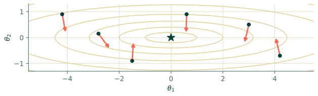
That last observation is important. The steepest direction is a purely local fact. In a long, narrow valley it points mostly across the valley, not along it, and following it step by step makes slow progress. This is the central difficulty of Section 3.2, and it returns in Part 4 as the reason PINN training is hard.

Minima, saddles and the shape of real landscapes

At a minimum the gradient is zero, but so it is at a maximum and at a saddle point (a pass between two hills, downhill in one direction and uphill in another). For the bowl above the only stationary point is the minimum, because the loss is convex. A neural network's loss is not convex: it has many stationary points and many different minima with different heights. In practice that is less fatal than it sounds, because in very high dimensions most stationary points are saddles that gradient methods eventually slide off, and many minima are nearly as good as one another. But it means that two runs from different starting points can end in different places, and that is why seeds and initialisation matter.

Exercises

1. For $\mathcal{L}(\theta) = \theta_1^2 + 3\theta_1\theta_2$, compute $\nabla\mathcal{L}$ and evaluate it at $(1, 1)$.
2. At that point, in which direction (as a unit vector) does the loss decrease fastest?
3. Is a point where the gradient is zero always a minimum?

Recap

• Parameters form a space; the loss is a height over it. The gradient is the vector of slopes, pointing uphill.
• $-\nabla\mathcal{L}$ is the direction of steepest descent, a local fact that need not point at the minimum.
• Network losses are not convex, so the end point depends on the start.