Generalisation: fitting is not understanding

The goal of learning is never to reproduce the training data. We already have the training data. The goal is to predict well at new inputs, and that ability is called generalisation.

Underfitting and overfitting

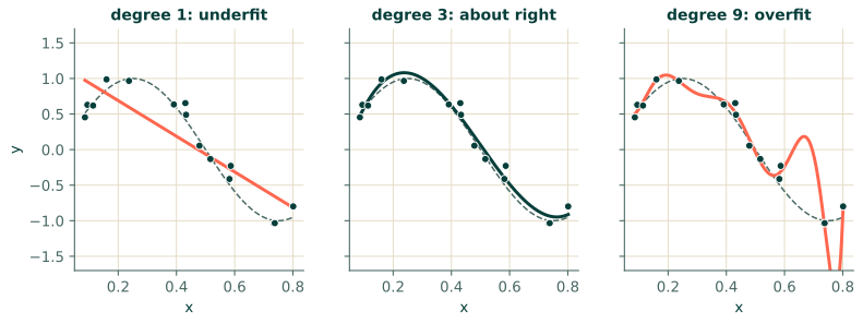
Give a model too little flexibility and it cannot capture the pattern: that is underfitting, like the straight line through a sine wave in Section 1.1. Give it too much and it can chase the noise, bending to pass through every measurement: that is overfitting.

We can measure both. Hold some data back, fit on the rest, and compare the loss on the two sets:

• Training loss: the error on the points the model was fitted to.
• Test loss: the error on fresh points from the same source, never used for fitting.

Let us run it. Same signal as before, $\sin(2\pi x)$ with noise of standard deviation $0.15$, fifteen training points, and 200 test points inside the same range. Four polynomial degrees:

import numpy as np

rng = np.random.default_rng(3)
x_tr = np.sort(rng.uniform(0, 1, 15))
y_tr = np.sin(2 * np.pi * x_tr) + 0.15 * rng.normal(size=15)
x_te = np.linspace(x_tr.min(), x_tr.max(), 200)
y_te = np.sin(2 * np.pi * x_te) + 0.15 * rng.normal(size=200)

def mse(c, x, y):
    return np.mean((np.polyval(c, x) - y) ** 2)

print("degree   train MSE   test MSE")
for d in [1, 3, 5, 9]:
    c = np.polyfit(x_tr, y_tr, d)
    print(f"{d:5d}   {mse(c, x_tr, y_tr):9.4f}   {mse(c, x_te, y_te):8.4f}")
print("noise floor (0.15**2):", 0.15 ** 2)

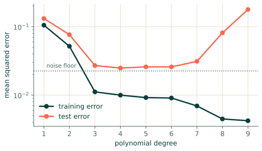
degree   train MSE   test MSE
    1      0.1051     0.1315
    3      0.0111     0.0270
    5      0.0092     0.0259
    9      0.0042     0.1779
noise floor (0.15**2): 0.0225

Read the two columns separately. The training error only ever goes down as the degree rises: a more flexible family can always fit the points at least as well. The test error goes down, bottoms out around degree 3 to 5, and then rises sharply. The degree-9 polynomial has almost memorised the fifteen points and pays for it everywhere in between.

There is also a floor. Because the test labels carry noise of their own, no model can score below $0.15^2 = 0.0225$ on them. A test error close to that floor means there is nothing left to learn.

Regularisation: a leash on flexibility

Choosing the degree is one way to control flexibility. Another is to keep a flexible model but penalise large parameters, which stops it from bending sharply. Add a term to the loss:

$$\mathcal{L}_\lambda(\theta) = \frac1N\sum_i \bigl(f_\theta(x_i) - y_i\bigr)^2 + \lambda\,\lVert\theta\rVert^2.$$

The number $\lambda \ge 0$ is a hyperparameter. At $\lambda = 0$ nothing changes; as it grows, the model is pulled towards small parameters and smoother curves. For this loss the normal equations of Section 1.2 just gain a term: $(X^\top X + N\lambda I)\,\theta = X^\top y$.

def ridge(x, y, degree, lam):
    X = np.vander(x, degree + 1)
    return np.linalg.solve(X.T @ X + len(x) * lam * np.eye(degree + 1), X.T @ y)

print("lambda      train MSE   test MSE   (degree 9)")
for lam in [0.0, 1e-8, 1e-6, 1e-4, 1e-2]:
    theta = ridge(x_tr, y_tr, 9, lam)
    print(f"{lam:8.0e}   {mse(theta, x_tr, y_tr):9.4f}   {mse(theta, x_te, y_te):8.4f}")

lambda      train MSE   test MSE   (degree 9)
   0e+00      0.0042     0.1777
   1e-08      0.0089     0.0257
   1e-06      0.0096     0.0247
   1e-04      0.0164     0.0325
   1e-02      0.0677     0.1105

The same degree-9 family that overfitted at $\lambda = 0$ becomes usable once it is held on a leash. (np.polyval accepts the coefficient vector from ridge directly because both use the highest power first.)

Never tune on the test set

One rule makes the difference between an honest number and a flattering one. If you choose the degree, or $\lambda$, by looking at the test error, the test set has become part of the training and the number it gives you is optimistic. The usual remedy is three-way splitting: train to fit $\theta$, validation to choose hyperparameters, and a test set touched once at the end.

In a PINN there is a natural version of this. After training, evaluate the equation's residual at points that were not used as collocation points. If it is small there as well, the network has learned the equation and not merely the places where you checked. Chapter 12 builds this check into the workflow.

Exercises

1. In the table above, which degree would you pick, and which column did you use to decide?
2. A student reports "training error 0.0001, so the model is excellent". What single further number do you need?
3. You double the number of training points to 30 but keep degree 9. Which of the two errors do you expect to change more, and why?

Recap

• Generalisation, not training error, is the measure that matters. Compare train and test loss.
• Too little flexibility underfits; too much overfits. Regularisation limits flexibility without changing the model family.
• In a PINN the equation is a regulariser that carries physical meaning, and held-out residuals are the test.

References

- Raissi, M., Perdikaris, P., & Karniadakis, G. E. (2019). Physics-informed neural networks: A deep learning framework for solving forward and inverse problems involving nonlinear partial differential equations. Journal of Computational Physics, 378, 686–707. doi:10.1016/j.jcp.2018.10.045