Learning a function from examples

Most programs are rules somebody wrote down. A rule for converting degrees Celsius to Fahrenheit is $F = 1.8\,C + 32$, and nothing is learned: the author knew the rule. Machine learning is for the other situation, where you have examples of what goes in and what comes out, and no rule you trust.

This book needs very little machine learning to get started, but it needs it precisely. This chapter fixes the vocabulary; the next two build the one tool, the neural network, that the rest of the book uses.

Data, model, parameters

Suppose we measure an unknown quantity $y$ at $N$ locations $x_1, \dots, x_N$. The measurements are our data:

$$\mathcal{D} = \{(x_i, y_i)\}_{i=1}^{N}.$$

We believe there is some underlying relationship $y = g(x)$ that we cannot write down, and that each measurement is a little off: $y_i = g(x_i) + \varepsilon_i$, where $\varepsilon_i$ is noise.

A model is a function $f_\theta(x)$ we can write down, with a list of numbers $\theta$ inside it that we are free to change. Those numbers are the parameters (also called weights). Different $\theta$ gives a different function. For example:

$$f_\theta(x) = \theta_0 + \theta_1 x \qquad\text{(a straight line, two parameters)}$$

$$f_\theta(x) = \theta_0 + \theta_1 x + \theta_2 x^2 + \theta_3 x^3 \qquad\text{(a cubic, four parameters)}.$$

Learning (also training or fitting) means choosing the $\theta$ for which $f_\theta$ matches the data well. How to say "well" in a single number is the subject of the next section. First, let us see the two models above try.

A first fit

We will use a signal we know the answer to, so that we can tell whether a model has found it: $g(x) = \sin(2\pi x)$ on $[0, 1]$, observed at twelve random points with a little noise added.

import numpy as np

rng = np.random.default_rng(0)
x = np.sort(rng.uniform(0, 1, 12))
y = np.sin(2 * np.pi * x) + 0.15 * rng.normal(size=x.size)

line = np.polyfit(x, y, deg=1)     # [slope, intercept]
cubic = np.polyfit(x, y, deg=3)    # [x^3, x^2, x, 1] coefficients

print("line  :", np.round(line, 2))
print("cubic :", np.round(cubic, 2))

line  : [-0.93  0.12]
cubic : [ 21.59 -32.06  11.    -0.26]

np.polyfit chose the parameters for us by minimising a loss that we will meet in the next section. Figure 1.1 shows both fits.

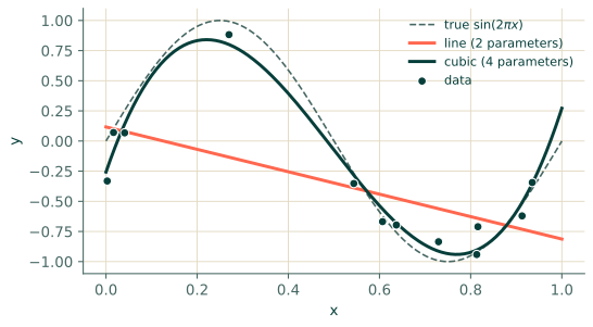
The line is a bad model for this data, however carefully its two parameters are chosen: no straight line looks like a sine wave. The cubic is much better. This is the first and most important fact about learning: how well you can do is limited by how flexible the family of functions is, before any question of how well you search it.

Parameters and hyperparameters

Two kinds of numbers appear when you train a model, and it is worth keeping them apart.

• Parameters $\theta$ are learned: the computer finds them. For a polynomial of degree $d$ there are $d + 1$ of them.
• Hyperparameters are chosen by you before training: the degree $d$, and later in this book the number of layers in a network, the learning rate, how many collocation points to use.

Choosing hyperparameters well is a large part of the craft, and a recurring theme of Part 4.

Regression, and why PINNs are regression

When the output is a number (or a vector of numbers) the task is called regression. When the output is a category ("cat" or "dog") it is classification. Everything in this book is regression: a PINN outputs the value of a physical field, such as a temperature, a displacement or a velocity, at any point you ask about.

Exercises

1. A polynomial model has degree 9. How many parameters does it have?
2. Without running anything: if the true relationship were exactly a straight line, would a cubic fit do worse than a line fit on noise-free data? Explain.

Recap

• Data are input–output pairs; a model is a function with adjustable parameters; training chooses them.
• The family of functions a model can represent limits the best possible fit.
• Parameters are learned, hyperparameters are chosen. A PINN is a regression model whose "data" can include an equation.

References

- Raissi, M., Perdikaris, P., & Karniadakis, G. E. (2019). Physics-informed neural networks: A deep learning framework for solving forward and inverse problems involving nonlinear partial differential equations. Journal of Computational Physics, 378, 686–707. doi:10.1016/j.jcp.2018.10.045