Scientific ML Studio

Section 2.1 ended with a claim: add up enough steps of the form $\tanh(wx + b)$ and you can build almost any shape. This section states the claim, tests it, and then lists what it does not promise.

The theorem

A network with one hidden layer and a scalar output is a sum of $H$ steps:

$$f_\theta(x) = \sum_{j=1}^{H} c_j\,\sigma\bigl(w_j x + b_j\bigr) + c_0.$$

Universal approximation. Take a continuous function $g$ on a closed interval (or, in several variables, on a closed bounded region), and any tolerance $\epsilon > 0$. Then for a suitable activation $\sigma$ there exists a number $H$ of hidden neurons and values of all the parameters such that $\lvert f_\theta(x) - g(x)\rvert < \epsilon$ for every $x$ in the region.

This was shown for sigmoidal activations by Cybenko (1989), and for a broad class of "squashing" activations (increasing functions that level off at both ends) by Hornik et al. (1989), whose title says it directly: multilayer feedforward networks are universal approximators. The result tells us that a neural network is not too weak a family of functions to even try. It is the reason the choice of model in a PINN is defensible.

Watching it happen

We can see the theorem work without any training at all. Pick the hidden weights $w_j, b_j$ at random, so the steps are scattered at random positions with random steepnesses, and then solve for the output weights $c_j$ by least squares. That last step is linear in $c$, so it is exactly the problem of Section 1.2.

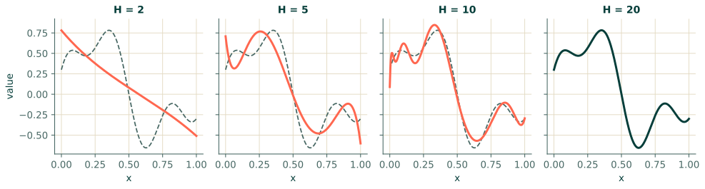
The target is a deliberately wiggly function, $g(x) = \sin(2\pi x)\,e^{-x} + 0.3\cos(5\pi x)$ on $[0, 1]$.

import numpy as np

g = lambda x: np.sin(2 * np.pi * x) * np.exp(-x) + 0.3 * np.cos(5 * np.pi * x)
xs = np.linspace(0, 1, 400)

def fit_random_features(H, seed=0):
    rng = np.random.default_rng(seed)
    w = 8 * rng.normal(size=H)             # random steepness and direction
    b = rng.uniform(-8, 8, size=H)         # random position
    features = np.tanh(np.outer(xs, w) + b)
    A = np.column_stack([features, np.ones_like(xs)])
    c, *_ = np.linalg.lstsq(A, g(xs), rcond=None)
    return A @ c

print(" H   max |f - g|")
for H in [2, 5, 10, 20, 40]:
    err = np.abs(fit_random_features(H) - g(xs)).max()
    print(f"{H:3d}   {err:.1e}")

 H   max |f - g|
  2   6.1e-01
  5   4.1e-01
 10   2.1e-01
 20   6.7e-04
 40   6.6e-05

With two neurons the worst-case error is as large as the function itself. With twenty it is below $10^{-3}$. Figure 2.5 shows the curves.

A wiggly target curve and four approximations built from 2, 5, 10 and 20 random tanh neurons; the fit improves with each increase until the curves are indistinguishable. — **Figure 2.5.** The target (dashed) and its approximation by $H$ tanh neurons whose positions were chosen at random. Only the output weights were fitted.

What the theorem does not say

The statement is an existence result, and a lot is hidden in the word "exists".

How many neurons? It gives no bound. For a hard function in many dimensions, $H$ can be astronomically large.
How to find the parameters? Nothing here says gradient descent will find them. Our demonstration cheated, in a good way: it chose the hidden layer at random and solved only the easy linear part. Full training of all parameters is a hard non-convex problem (Chapter 3).
Derivatives. Approximating $g$ closely does not mean approximating $g'$ or $g''$ closely. A function can be within $10^{-6}$ of $g$ everywhere and still have a wildly different slope. A PINN's residual depends on exactly those derivatives, so the guarantee does not by itself cover what a PINN needs.
Away from the data. The theorem is about a fixed region. It says nothing about how a network trained on samples behaves between them, or outside.

Reading the theorem as a promise

"A neural network can represent any function" is true and, by itself, nearly useless for engineering. The questions that decide whether a PINN works are about optimisation, scaling and sampling, which is why most of this book is about those and not about expressive power.

Depth

The theorem is about a single hidden layer, yet practical networks use several. Depth does not enlarge the class of representable functions (one layer is already universal) but it can make some functions representable with far fewer neurons overall, by composing simple pieces. Whether that helps for a given physical problem is, again, an empirical question that Part 4 revisits.

Exercises

In the experiment, the number of free parameters at width $H$ is $H$ output weights plus one bias that are fitted. How many is that for $H = 20$?
Suppose a network matches a function to within $10^{-3}$ everywhere. Can you conclude its second derivative is within $10^{-3}$ of the function's second derivative?
Why is the demonstration not "training a neural network"?

Answers

21 fitted numbers ($H$ output weights and one constant). The $2H = 40$ hidden weights and biases were drawn at random and never adjusted.
No. Small differences in value can come with large differences in slope or curvature, for example $10^{-3}\sin(10^{4}x)$ has size $10^{-3}$ and second derivative of size $10^{5}$.
Because only the last layer was fitted, and that part is linear. Real training adjusts every weight, including those inside the non-linearities.

Recap

One hidden layer of enough smooth neurons can approximate any continuous function on a bounded region (Cybenko, 1989; Hornik et al., 1989).
The result is existence only: no size bound, no recipe for the parameters, and no guarantee on derivatives.
Practical success depends on optimisation, sampling and architecture, which is where the rest of the book spends its time.

What a network can represent

References

- Cybenko, G. (1989). Approximation by superpositions of a sigmoidal function. Mathematics of Control, Signals and Systems, 2(4), 303–314. doi:10.1007/bf02551274
- Hornik, K., Stinchcombe, M., & White, H. (1989). Multilayer feedforward networks are universal approximators. Neural Networks, 2(5), 359–366. doi:10.1016/0893-6080(89)90020-8