Adaptive refinement
The residual tells you where the network is wrong, without knowing the answer. Moving points there is a way of re-weighting the loss, and for a solution with a sharp feature it decides whether the feature is found at all.
An even spread of points (Section 7.1) treats every part of the domain as equally important. Many solutions are not like that: a shock, a boundary layer or a steep front occupies a small part of the domain and carries most of the difficulty. Section 6.5 showed that the residual can be evaluated anywhere, for free, without a reference solution. That makes it an error indicator: a map of where the network is struggling, which can be used to decide where the next points should go.
Re-weighting by moving points
Section 6.1 read the equation term as a Monte Carlo estimate of an integral. That reading says what moving the points does. If the collocation points are drawn from a probability density $p(\mathbf{x})$ on the domain, then
$$\frac{1}{N}\sum_{i=1}^{N} r_\theta(\mathbf{x}_i)^2 \;\approx\; \int_\Omega r_\theta(\mathbf{x})^2\, p(\mathbf{x})\,d\mathbf{x},$$
so the loss weights each part of the domain by the density of points there. Uniform points weigh every part equally. Points concentrated where $|r_\theta|$ is large weigh the loss towards the places where the network is wrong. Redrawing uniform points more often, as in Section 7.1, changes which points are used, but not this weighting: on average it is still the uniform integral.
Three methods are in wide use, all of them loops of "train for a while, look at the residual, move the points":
| Method | What happens at each refinement | Number of points |
|---|---|---|
| RAR, residual-based adaptive refinement (Lu et al., 2021) | evaluate $|r_\theta|$ at many random candidates and add the few with the largest residual | grows |
| RAD, residual-based adaptive distribution (Wu et al., 2023) | redraw all the points, with probability $p(\mathbf{x}) \propto \dfrac{|r_\theta(\mathbf{x})|^k}{\operatorname{mean}|r_\theta|^k} + c$ | fixed |
| R3, retain, resample, release (Daw et al., 2023) | keep the points whose residual is above average, replace the others by fresh uniform points | fixed |
RAD has two settings. The exponent $k$ says how sharply the points concentrate on the largest residuals: $k = 0$ gives uniform redraws, and a large $k$ approaches RAR's choice of only the worst points. The floor $c$ keeps some points everywhere, so that regions which are currently fine are not abandoned: the larger $c$, the more uniform the draw. Wu et al. (2023) compared these and other strategies over thousands of runs and suggest $k = 1$, $c = 1$ as a good default for RAD. R3 was designed against propagation failures, in which the correct solution does not spread from the initial and boundary conditions into the rest of the domain, a failure typical of evolution problems (Section 8.2).
A sharp layer
The test problem has a solution that is flat almost everywhere and jumps from $-1$ to $+1$ over a width of about a tenth, around $x = 0.4$:
$$-u'' = f \ \text{ on } (0, 1), \qquad u(x) = \tanh\!\left(\frac{x - 0.4}{\delta}\right), \quad \delta = 0.02,$$
with $f$ worked out from $u$ and the boundary values taken from $u$. The source $f$ is of order $1/\delta^2 = 2500$ inside the layer and almost zero outside, so the residual is divided by that natural size (Section 4.5). Every run below uses the same network (three hidden layers of 32 tanh neurons), the same optimiser (Adam, learning rate $10^{-3}$, 10000 epochs) and at most 64 collocation points, chosen in one of five ways:
- fixed: 64 uniform random points, drawn once;
- redrawn: 64 fresh uniform points at every epoch, the Studio's Resample points every set to 1;
- RAR: 32 uniform points to start with; every 500 epochs, the 4 worst of 1000 random candidates are added, up to 64;
- RAD (1, 1) and RAD (2, 0): 64 points, redrawn every 500 epochs from 1000 random candidates, with $(k, c)$ as given.
import math
import torch
import torch.nn as nn

def d(y, x):
    return torch.autograd.grad(y, x, torch.ones_like(y), create_graph=True)[0]

delta, x0 = 0.02, 0.4                                         # width and position of the layer
s = lambda x: (x - x0) / delta
exact = lambda x: torch.tanh(s(x))
f = lambda x: 2 / delta**2 * torch.tanh(s(x)) / torch.cosh(s(x)) ** 2      # -u'' for the exact u
residual = lambda u, x: (-d(d(u(x), x), x) - f(x)) * delta**2              # divided by its natural size
x_b = torch.tensor([[0.0], [1.0]])
x_test = torch.linspace(0, 1, 4001).reshape(-1, 1)

def refine(mode, u, x_col):
    """Choose the next collocation points from 1000 random candidates, using the residual."""
    candidates = torch.rand(1000, 1).requires_grad_(True)
    r = residual(u, candidates).detach().abs().flatten()
    candidates = candidates.detach()
    if mode == "RAR":                                         # add the 4 worst candidates
        return torch.cat([x_col, candidates[r.topk(4).indices]])
    k, c = {"RAD (1, 1)": (1, 1), "RAD (2, 0)": (2, 0)}[mode]
    p = r**k / (r**k).mean() + c                              # redraw every point from this density
    return candidates[torch.multinomial(p / p.sum(), len(x_col), replacement=False)]

def train(mode, seed, epochs=10000, every=500):
    torch.manual_seed(seed)
    net = nn.Sequential(nn.Linear(1, 32), nn.Tanh(), nn.Linear(32, 32), nn.Tanh(),
                        nn.Linear(32, 32), nn.Tanh(), nn.Linear(32, 1))
    u = lambda x: net(2 * x - 1)
    x_col = torch.rand(32 if mode == "RAR" else 64, 1)       # RAR starts with half the points
    opt = torch.optim.Adam(net.parameters(), lr=1e-3)
    errors = []
    for epoch in range(1, epochs + 1):
        if mode == "redrawn":
            x_col = torch.rand(64, 1)
        x = x_col.clone().requires_grad_(True)
        opt.zero_grad()
        loss = (residual(u, x) ** 2).mean() + ((u(x_b) - exact(x_b)) ** 2).sum()
        loss.backward()
        opt.step()
        adaptive = mode.startswith("RAD") or (mode == "RAR" and len(x_col) < 64)
        if adaptive and epoch % every == 0 and epoch < epochs:
            x_col = refine(mode, u, x_col)
        if epoch % 5000 == 0:
            with torch.no_grad():
                errors.append(((u(x_test) - exact(x_test)).norm() / exact(x_test).norm()).item())
    return errors, x_col

modes = ["fixed", "redrawn", "RAR", "RAD (1, 1)", "RAD (2, 0)"]
runs = {mode: [train(mode, seed) for seed in range(3)] for mode in modes}

print("relative L2 error     after 5000 epochs (seeds 0, 1, 2)    after 10000 epochs")
for mode in modes:
    at_5000 = "  ".join(f"{errors[0]:.1e}" for errors, _ in runs[mode])
    at_10000 = "  ".join(f"{errors[1]:.1e}" for errors, _ in runs[mode])
    print(f"{mode:12s}          {at_5000}            {at_10000}")
relative L2 error     after 5000 epochs (seeds 0, 1, 2)    after 10000 epochs
fixed                 4.8e-01  5.4e-01  5.0e-01            3.2e-02  4.8e-01  4.4e-02
redrawn               5.0e-01  5.4e-01  5.2e-01            2.4e-02  4.6e-01  2.2e-01
RAR                   1.9e-02  1.2e-01  4.9e-02            5.5e-02  6.0e-02  2.4e-02
RAD (1, 1)            3.8e-02  5.3e-01  4.6e-01            1.4e-02  3.0e-02  2.7e-02
RAD (2, 0)            3.4e-02  5.6e-02  7.7e-02            1.5e-02  1.8e-02  7.1e-02
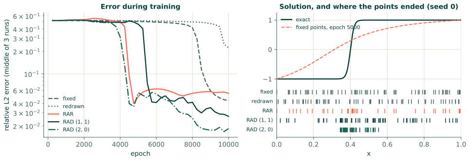
Read the table by counting the runs that found the layer. An error of a few per cent means the jump is in place; an error near 50% means the network has drawn a smooth curve through it instead (the dashed line in Figure 7.2). After 5000 epochs no uniform run, fixed or redrawn, has found the layer. Every RAR and RAD (2, 0) run has, and one of the three RAD (1, 1) runs. After 10000 epochs every adaptive run has found it, against two of the three fixed runs and one of the redrawn ones, with a second redrawn run part of the way there.
Once the layer is found, the errors are much alike, between about 1.5 and 7 per cent, whichever way the points were chosen. What adaptive sampling bought here is reliability and speed rather than a better final answer: the uniform sets can find the layer, but only some of the time and late. The greediest settings, RAR and RAD (2, 0), found it soonest. Redrawing uniform points every epoch did no better than keeping them fixed, as the weighting argument predicts.
Where did the points go? The layer, $|x - 0.4| < 0.1$, is a fifth of the interval, so a fifth of a uniform set falls in it:
for mode in modes:
    x_col = runs[mode][0][1]                                  # the final points of the seed-0 run
    near = ((x_col - x0).abs() < 0.1).float().mean().item()
    print(f"{mode:12s}  {len(x_col):3d} points,  {near:4.0%} of them within 0.1 of the layer")
fixed          64 points,   22% of them within 0.1 of the layer
redrawn        64 points,   14% of them within 0.1 of the layer
RAR            64 points,   61% of them within 0.1 of the layer
RAD (1, 1)     64 points,   38% of them within 0.1 of the layer
RAD (2, 0)     64 points,   91% of them within 0.1 of the layer
RAR and RAD (2, 0) moved most of their points into the layer, three fifths and nine tenths of them, against a fifth for a uniform set. RAD (1, 1) moved fewer, keeping the rest spread over the flat parts, which is what its floor $c$ is for. A uniform set would need about 200 to 300 points to put as many in the layer as these 64 do.
What it costs, and what it cannot see
Each refinement evaluates the residual at the candidates once: here 1000 points every 500 epochs, a small fraction of the cost of training. Three other prices are easier to miss.
- The loss changes meaning. After each refinement the loss is measured at different points, so it jumps, and loss curves from adaptive runs cannot be compared with each other or used for early stopping. Judge them by the residual at a fixed set of fresh points (Section 6.5) or by a reference.
- Greedy choices abandon the rest of the domain. Points piled on the worst spot leave the smooth parts with few points, and the error can grow there unseen. RAD's floor $c$, R3's fresh uniform points, or simply keeping a uniform core set, prevent this.
- The residual only sees the equation. An error that comes from a missing or wrong condition does not make the residual large anywhere. In Section 6.3 the runs with a slope at both ends were wrong by a constant while the residual was small everywhere: no placement of points can fix a problem that does not define the answer.
In the Studio
The Studio's Train block offers Resample points every, which redraws the interior points uniformly: the
"redrawn" strategy above, which is not adaptive. Adaptive sampling is a few lines added to a generated script,
because the training loop draws all of its interior points through one function, sample_interior, and looks
that function up every time it resamples. For the 1D Poisson script:
# not run
import torch
import poisson_1d as p                                  # the generated script, saved as poisson_1d.py

uniform_points = p.sample_interior                      # keep the generated sampler

def rad_points(n=p.N_INTERIOR, strategy=p.INTERIOR_STRATEGY, k=1.0, c=1.0):
    """RAD: n points drawn from ten times as many candidates, by p ~ |r|^k / mean(|r|^k) + c."""
    candidates = uniform_points(10 * n, strategy)
    r = p.residual_pde1(candidates).detach().abs().flatten() ** k
    weights = r / r.mean() + c
    keep = torch.multinomial(weights / weights.sum(), n, replacement=False)
    return candidates[keep].detach().requires_grad_(True)

p.sample_interior = rad_points
p.RESAMPLE_EVERY = 500                                  # redraw every 500 epochs
history = p.train()
The residual function is named after the PDE block, residual_pde1 for the first one; a script with several
equations has one function for each, and the weights can use their sum. On a smooth solution like this one there
is little for it to find; it pays off on solutions like the one above.
Exercises
- In RAD with $k = 1$ and $c = 1$, what fraction of the points is, on average, drawn as if uniformly?
- Why does RAR add a few points at a time rather than all of its budget at the first refinement?
- A run with RAD has a loss curve that rises sharply every 500 epochs. Is something wrong?
Answers
- Half. Over the domain, $|r|^k/\operatorname{mean}|r|^k$ averages to 1, and so does $c = 1$; the density is an equal mixture of the two, so on average half the points come from the uniform part.
- The worst residuals cluster around the single worst place. Adding the whole budget at once piles every point there before the network has had a chance to respond, and the next-worst region gets nothing. Adding a few at a time lets the residual map, and so the choice, change as the network improves.
- Not necessarily. Each redraw moves the points to where the residual is largest, so the loss measured right after the redraw is larger by design. Judge progress by the residual at a fixed set of test points, or the error against a reference.
Recap
- Collocation points drawn from a density $p$ make the loss an integral weighted by $p$: moving points re-weights the loss. Redrawing uniform points does not change the weighting.
- RAR adds the worst candidates, RAD redraws all points from a residual-based density, and R3 keeps the worst and refreshes the rest.
- On a sharp layer, adaptive sampling found the layer sooner and more reliably than any uniform set of the same size. It cannot repair a badly posed problem, and it makes the loss curve harder to read.
References
- Daw, A., Bu, J., Wang, S., Perdikaris, P., & Karpatne, A. (2023). Mitigating propagation failures in physics-informed neural networks using retain-resample-release (R3) sampling. Proceedings of the 40th International Conference on Machine Learning, 202, 7264–7302. https://proceedings.mlr.press/v202/daw23a.html
- Lu, L., Meng, X., Mao, Z., & Karniadakis, G. E. (2021). DeepXDE: A deep learning library for solving differential equations. SIAM Review, 63(1), 208–228. doi:10.1137/19M1274067
- Wu, C., Zhu, M., Tan, Q., Kartha, Y., & Lu, L. (2023). A comprehensive study of non-adaptive and residual-based adaptive sampling for physics-informed neural networks. Computer Methods in Applied Mechanics and Engineering, 403, 115671. doi:10.1016/j.cma.2022.115671