Three ways to take a derivative
By hand, by finite differences, or automatically. Only the third is both exact and cheap for a neural network, and the reasons why are the reasons a PINN is possible.
A PINN's loss contains derivatives of the network with respect to its inputs: $u_x$, $u_t$, $u_{xx}$. They have to be computed at thousands of points, at every training step, accurately enough that the residual means something. There are three ways a computer can take a derivative. This section tries all three on the same functions and measures what each one costs and how wrong it is.
By hand, on a computer: symbolic differentiation
A computer algebra system such as SymPy applies the rules of calculus to a formula and returns a new formula. The answer is exact. The trouble is size. Write a tiny network, one input, two hidden layers of three tanh neurons and one output, as a formula with its weights filled in, and differentiate it repeatedly:
import numpy as np
import sympy as sp

rng = np.random.default_rng(0)
x = sp.symbols("x")
W1, b1 = np.round(rng.normal(size=3), 2), np.round(rng.normal(size=3), 2)
W2, b2 = np.round(rng.normal(size=(3, 3)), 2), np.round(rng.normal(size=3), 2)
W3 = np.round(rng.normal(size=3), 2)

h1 = [sp.tanh(sp.Float(W1[i]) * x + sp.Float(b1[i])) for i in range(3)]
h2 = [sp.tanh(sum(sp.Float(W2[i, j]) * h1[j] for j in range(3)) + sp.Float(b2[i])) for i in range(3)]
u = sum(sp.Float(W3[j]) * h2[j] for j in range(3))

for k in range(4):
    print(f"derivative {k}: {sp.count_ops(sp.diff(u, x, k)):5d} operations")
derivative 0:    53 operations
derivative 1:   116 operations
derivative 2:   329 operations
derivative 3:  1070 operations
Every derivative is a longer formula than the last, because the product and chain rules turn one term into several. This is called expression swell. A network of the size a PINN uses, with four layers of forty neurons, would produce formulas far too large to be useful. Symbolic differentiation is the right tool for manufacturing a source term (Section 4.4) and the wrong one for a network.
By finite differences
The second way needs no formula at all, only the ability to evaluate the function. The central differences
$$u'(x) \approx \frac{u(x + h) - u(x - h)}{2h}, \qquad u''(x) \approx \frac{u(x + h) - 2u(x) + u(x - h)}{h^2}$$
have errors proportional to $h^2$, so a smaller step should be better. It is, up to a point. Each evaluation of $u$ carries a rounding error of about $\epsilon\,|u|$, where $\epsilon$ is the machine precision ($2.2\times10^{-16}$ in 64-bit floating point, $1.2\times10^{-7}$ in 32-bit), and the formulas divide that error by $h$ or by $h^2$. Shrinking $h$ trades truncation error for rounding error. Here is the trade, measured on $u = \sin(\pi x)$, whose derivatives we know, as the worst error over 91 points:
xs = np.linspace(0.05, 0.95, 91)
exact1, exact2 = np.pi * np.cos(np.pi * xs), -np.pi**2 * np.sin(np.pi * xs)

print("     h    first, float64  second, float64  first, float32  second, float32")
for h in [1e-1, 1e-2, 1e-3, 1e-4, 1e-5, 1e-6, 1e-7]:
    row = []
    for dtype in (np.float64, np.float32):
        x_, h_, pi = xs.astype(dtype), dtype(h), dtype(np.pi)
        f = lambda z: np.sin(pi * z)
        d1 = (f(x_ + h_) - f(x_ - h_)) / (2 * h_)
        d2 = (f(x_ + h_) - 2 * f(x_) + f(x_ - h_)) / (h_ * h_)
        row += [np.abs(d1 - exact1).max(), np.abs(d2 - exact2).max()]
    print(f"{h:7.0e}  " + "  ".join(f"{e:15.1e}" for e in row))
     h    first, float64  second, float64  first, float32  second, float32
  1e-01          5.1e-02          8.1e-02          5.1e-02          8.1e-02
  1e-02          5.1e-04          8.1e-04          5.1e-04          2.6e-03
  1e-03          5.1e-06          8.1e-06          8.2e-05          2.8e-01
  1e-04          5.1e-08          1.0e-07          7.9e-04          2.3e+01
  1e-05          5.2e-10          4.6e-06          7.1e-03          2.1e+03
  1e-06          2.1e-10          4.7e-04          8.3e-02          2.4e+05
  1e-07          3.0e-09          4.5e-02          1.5e+00          2.7e+07
Read down each column (Figure 5.1 draws them). In 64-bit arithmetic the first derivative improves until
$h \approx 10^{-6}$ and the second until $h \approx 10^{-4}$, then both get worse. In 32-bit arithmetic, which
is PyTorch's default, the second derivative is never better than about $10^{-3}$, that is $10^{-4}$ relative to
its size, and at $h = 10^{-5}$ it is wrong by more than a thousand. A PINN that formed $u_{xx}$ this way in
float32 would be fitting rounding noise.
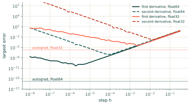
There is a second cost. Every finite-difference derivative needs extra evaluations of the function: two for a first derivative, three for a second, more in several dimensions, and each is a full forward pass of the network.
Automatically
The third way is automatic differentiation. It does not manipulate formulas and it does not take small steps. A program that evaluates a network is a sequence of elementary operations: multiply, add, tanh. Each has a derivative that is known exactly. Automatic differentiation records the sequence while it runs and then applies the chain rule to it, operation by operation, with numbers rather than formulas (Baydin et al., 2018; Griewank & Walther, 2008). The result is the exact derivative of the function the program computes, wrong only by rounding:
import torch

for dtype in (torch.float64, torch.float32):
    x_ = torch.tensor(xs, dtype=dtype, requires_grad=True)
    u_ = torch.sin(torch.pi * x_)
    ux, = torch.autograd.grad(u_.sum(), x_, create_graph=True)
    uxx, = torch.autograd.grad(ux.sum(), x_)
    print(f"autograd, {str(dtype)[6:]:8s}  first {np.abs(ux.detach().numpy() - exact1).max():.1e}"
          f"   second {np.abs(uxx.numpy() - exact2).max():.1e}")
autograd, float64   first 0.0e+00   second 1.8e-15
autograd, float32   first 7.1e-07   second 2.1e-06
The errors are at the level of the arithmetic itself, in either precision, for the first derivative and the second alike. There is no step to choose. The cost is a small multiple of one evaluation, as Section 3.4 found for gradients with respect to the weights, and Section 5.2 shows why.
| Method | Accuracy | Cost per derivative | Works on a network? |
|---|---|---|---|
| Symbolic | exact | grows with the size of the formula | only for tiny ones |
| Finite differences | $h^2$ truncation plus rounding amplified by $1/h$ or $1/h^2$ | extra evaluations per point and per direction | yes, inaccurately |
| Automatic | exact up to rounding | a small multiple of one evaluation | yes |
Where this goes in a PINN
"Exact" here means the exact derivative of the network, not of the true solution. Automatic differentiation removes the error of taking the derivative; it does nothing about the network being an approximation. That second error is what training reduces, and what Chapter 6 measures. Without the first error gone, the second could not even be measured. It is why Raissi et al. (2019) built PINNs on automatic differentiation and not on a finite-difference stencil.
Exercises
- For a central first difference in 64-bit arithmetic, the truncation error is about $h^2|u'''|/6$ and the rounding error about $\epsilon|u|/h$. Find the $h$ that balances them for $u = \sin(\pi x)$, roughly. Does it match the table?
- Why is a 32-bit second difference so much worse than a 32-bit first difference at the same $h$?
- A colleague proposes computing $u_{xx}$ for a PINN by finite differences in
float64with $h = 10^{-4}$, to avoid "complicated autograd". Give two reasons against.
Answers
- Setting $h^2\pi^3/6 \approx \epsilon/h$ gives $h^3 \approx 6\epsilon/\pi^3 \approx 4\times10^{-17}$, so $h \approx 3\times10^{-6}$. The table's best first derivative is at $h = 10^{-6}$ to $10^{-5}$. Yes.
- The rounding error of the second difference is divided by $h^2$, not $h$, and 32-bit rounding is about $5\times10^{8}$ times larger than 64-bit. At $h = 10^{-3}$, $\epsilon/h^2 \approx 10^{-7}/10^{-6} = 0.1$: an error of order one tenth, as the table shows.
- It costs three network evaluations per point and per direction instead of one pass and a backward sweep,
and its accuracy (about $10^{-7}$ at best) puts a floor under the residual that training cannot get below.
It also forces the whole network into
float64, which costs memory and time, whereas autograd is accurate to about $10^{-6}$ even infloat32.
Recap
- Symbolic differentiation is exact but its formulas swell; finite differences are simple but trade truncation against rounding, disastrously for second derivatives in 32-bit arithmetic.
- Automatic differentiation applies the chain rule to the recorded computation: exact up to rounding, for a small multiple of the cost of one evaluation.
- It gives the exact derivative of the network. Whether the network is close to the solution is a separate question, and the one training answers.
References
- Baydin, A. G., Pearlmutter, B. A., Radul, A. A., & Siskind, J. M. (2018). Automatic differentiation in machine learning: a survey. Journal of Machine Learning Research, 18(153), 1–43. https://jmlr.org/papers/v18/17-468.html
- Griewank, A., & Walther, A. (2008). Evaluating derivatives: Principles and techniques of algorithmic differentiation. Society for Industrial and Applied Mathematics. 2nd edition. doi:10.1137/1.9780898717761
- Raissi, M., Perdikaris, P., & Karniadakis, G. E. (2019). Physics-informed neural networks: A deep learning framework for solving forward and inverse problems involving nonlinear partial differential equations. Journal of Computational Physics, 378, 686–707. doi:10.1016/j.jcp.2018.10.045