A shock wave: Burgers' equation and the second optimiser
A smooth start turns into a near-vertical jump. See why Adam alone gets stuck, how a second stage with L-BFGS fixes it, and how to grade an answer when the reference is a numerical integral and not a formula.
All the equations so far were linear. Doubling the solution doubled the answer, and the exact solution was a neat product of sines and exponentials. Burgers' equation is the first nonlinear problem in this series. Its solution starts as a gentle sine wave and steepens, until a nearly vertical jump appears in the middle: a shock.
It is the classic stress test for PINNs, and it teaches three lessons the earlier guides could not: what a nonlinear term does to the loss, why a second optimiser stage is often the difference between a poor answer and a good one, and how to build a reference solution when no simple formula exists.
Before you start. Finish Heat in a bar and A standing wave first. Open the Studio and choose an empty canvas.
1. The problem
Let $u(x,t)$ be a velocity along a line. Burgers' equation says that the velocity is carried along by itself, while a little friction smooths things out:
$$ \frac{\partial u}{\partial t} + u\,\frac{\partial u}{\partial x} = \nu\,\frac{\partial^2 u}{\partial x^2}, \qquad -1 < x < 1,\quad 0 < t \le 1, $$
with a small viscosity $\nu = 0.01/\pi \approx 0.0032$. The start is a sine wave, and the ends are held at zero:
$$ u(x,0) = -\sin(\pi x), \qquad u(-1,t) = 0, \qquad u(1,t) = 0 . $$
Why a shock appears
The term $u\,u_x$ says that every point on the profile moves at its own value of $u$. Where $u$ is positive, the profile moves right; where it is negative, left. The initial wave $-\sin(\pi x)$ is positive on the left half and negative on the right half, so the two sides rush towards the middle and pile up. Without friction they would form a true discontinuity in finite time. With friction $\nu$ they form a very thin steep layer instead, which is the shock. Smaller $\nu$ means a thinner shock and a harder problem. The value $0.01/\pi$ is a standard benchmark in the PINN literature.
The reference solution
There is a neat exact route even though no simple formula exists. The Cole–Hopf transform turns Burgers' equation into the plain heat equation, and the answer comes out as a ratio of two integrals:
$$ u(x,t) = -\,\frac{\displaystyle\int_{-\infty}^{\infty} \sin\bigl(\pi(x-\eta)\bigr)\, f(x-\eta)\, e^{-\eta^{2}/(4\nu t)}\, d\eta}{\displaystyle\int_{-\infty}^{\infty} f(x-\eta)\, e^{-\eta^{2}/(4\nu t)}\, d\eta}, \qquad f(y) = e^{-\cos(\pi y)/(2\pi\nu)} . $$
You do not need to follow the derivation. What matters is that this can be evaluated by numerical integration to high accuracy at any point, so it works as a trustworthy reference. The reference script does it with a fine trapezoid sum. As a sanity check, it was compared against an independent finite-difference solution at several times; the two agreed to about $10^{-3}$ at the sampled points, a gap that comes from the finite-difference grid and not from the reference.
Why this matters beyond Burgers. A PINN is only worth trusting when it has been compared against something independent. Sometimes that is an exact formula (earlier guides), sometimes a finite element or finite difference solution (the Poisson guide), and sometimes, as here, an integral that a computer can evaluate. The habit is the same every time.
2. How a PINN sees the problem
The network is $u_\theta(x,t)$ with two inputs. The residual now contains the unknown multiplied by its own derivative:
$$ r_\theta(x,t) = \frac{\partial u_\theta}{\partial t} + u_\theta\,\frac{\partial u_\theta}{\partial x} - \nu\,\frac{\partial^2 u_\theta}{\partial x^2}. $$
That product is what makes the problem nonlinear. In practice it changes very little in the Studio, because automatic differentiation does not care. What it changes is the difficulty of the optimisation: the loss surface is much more awkward, with long flat valleys that gradient-based training crawls along.
$$ \mathcal{L}(\theta) = \overline{r_\theta^{\,2}} + w_{\text{ic}}\,\overline{\bigl(u_\theta(x,0) + \sin\pi x\bigr)^2} + w_{\text{bc}}\,\overline{u_\theta^{\,2}}_{\text{ends}} . $$
3. The plan: one block per decision
| # | Block | The question it answers | Our choice |
|---|---|---|---|
| 1 | DOM Domain | Where does the problem live? | One space dimension, $x\in[-1,1]$, time on, $t\in[0,1]$ |
| 2 | PDE Equation | Which equation must hold inside? | Burgers, $u_t + u\,u_x = \nu\,u_{xx}$, with $\nu = 0.01/\pi$ |
| 3 | BC Boundary | What is fixed at the ends and at the start? | $u(-1,t)=0$, $u(1,t)=0$, initial profile $-\sin(\pi x)$ |
| 4 | NET Network | What function family do we search in? | 2 inputs, 8 hidden layers of 20 neurons, $\tanh$, 1 output |
| 5 | LOSS Loss | How do we score the errors? | Mean squared error, weight 1 on the PDE and 10 on every constraint |
| 6 | OPT Optimiser | How do the weights change? | Adam at $10^{-3}$ for 3000 epochs, then L-BFGS for 3000 iterations |
| 7 | RUN Train | How long and with how many points? | About 10000 interior points, 200 on each end, 400 at $t=0$ |
A note on labels. The Studio's wording can differ slightly between versions. The quantity to set is what matters; if a field name does not match exactly, pick the nearest one. If your version offers the second-stage optimiser under a different name, it is the option that names L-BFGS. If a value is not offered, keep the Studio's default.
The network is deeper and narrower than before, and there are far more points. A shock is a sharp feature, and a small, shallow network struggles to bend steeply enough, so the extra depth and the ten thousand points are not a luxury here.
4. Step by step in the Studio
Step 1: Domain (DOM)
Add a Domain block: one-dimensional, $x$ from −1 to 1 (note the symmetric interval), time on, $t$ from 0 to 1.
Step 2: Equation (PDE)
Add an Equation block, connect the Domain, and choose Burgers. Set the viscosity $\nu$ to 0.01/pi.
Check: the summary reads $u_t + u\,u_x = \nu\,u_{xx}$ with $\nu \approx 0.00318$. A common slip is to enter 0.01 and not 0.01/pi, which gives a viscosity three times too large and a visibly smoother, wrong shock.
Step 3: Boundary and initial conditions (BC)
Add a Boundary block, connect the Domain, and enter three conditions:
| Where | Type | Value |
|---|---|---|
| $x = -1$ | Fixed value (Dirichlet) | $u = 0$ |
| $x = 1$ | Fixed value (Dirichlet) | $u = 0$ |
| $t = 0$ | Initial condition | -sin(pi*x) |
Check: the Studio counts three conditions. Mind the minus sign in the initial condition. Without it the wave runs the other way and the shock forms in the same place, but the picture is mirrored and the comparison fails.
Step 4: Network (NET)
Add a Network block, connect the Domain, and use 2 inputs, 8 hidden layers of 20 neurons, tanh, and 1 output.
Step 5: Loss (LOSS)
Add a Loss block, connect the Equation, Boundary and Network, use mean squared error, set the PDE weight to 1 and the constraints to 10. If the Studio asks for the boundary weights as a list in the order above, enter [10, 10, 10].
Step 6: Optimiser (OPT), two stages
This is the step that matters most in this guide. Add an Optimiser block and set the first stage to Adam, learning rate 0.001, 3000 epochs. Then switch on the second stage and choose L-BFGS, with 3000 iterations.
Why two stages? Adam is the reliable general-purpose choice. It takes cheap, noisy steps, copes with badly scaled problems and gets you into the right region quickly. L-BFGS is a quasi-Newton method: it uses curvature information to take far more careful steps, and it can walk down a long narrow valley that Adam crawls along. It is slow and fragile on its own, but excellent as a finishing stage.
Step 7: Train (RUN)
Add a Train block, connect the Loss and Optimiser, and set about 10000 interior points.
Check: no warnings. A clean check means consistent, not accurate.
Step 8: Generate and run
Generate the Python code, download the script and run it on your own computer. The Studio builds and checks the configuration; training happens in your script. This is the most expensive run in the series: expect it to take on the order of ten to twenty minutes on a laptop CPU, most of it in the L-BFGS stage.
Step 9: Judge the result
The reference solution comes from the Cole–Hopf integral above, evaluated on a $201\times101$ grid in $(x,t)$ that was not used for training.
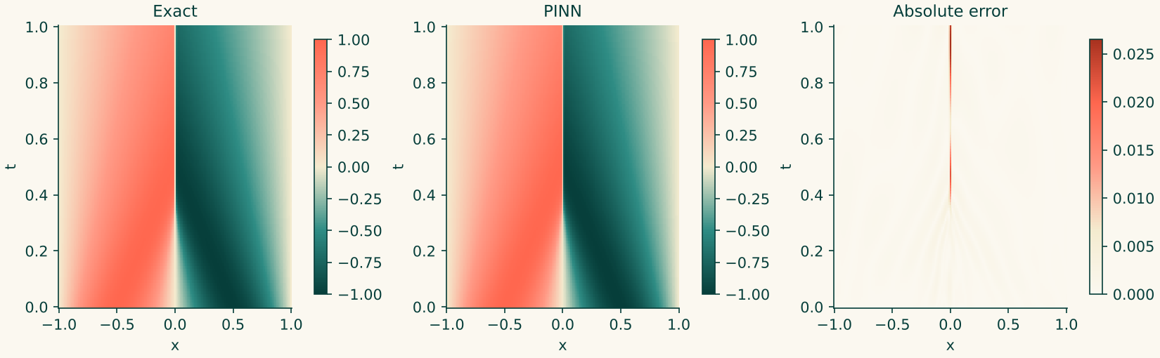
The first two panels are the same picture: a wave that steepens into a sharp line down the middle by about $t=0.5$. The error panel shows exactly what you would predict. It is tiny everywhere except along the shock. In the reference run the largest error inside $|x|<0.1$ was about $2.6\times10^{-2}$, while everywhere else it was $2.3\times10^{-3}$ or less.
Snapshots show it more directly. The solid line is the reference and the dashed line the PINN:
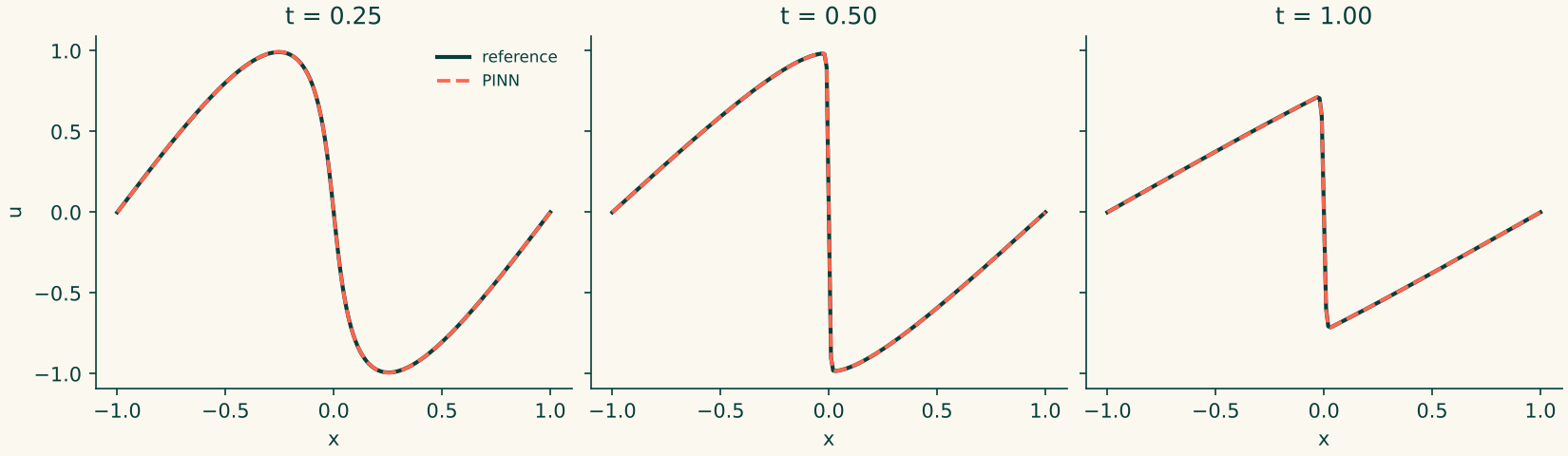
At $t=0.25$ the profile is still smooth. By $t=0.5$ the jump is almost vertical, and at $t=1$ the two halves have become straight ramps that meet at a small jump. The PINN follows all three closely. A sharper test: the steepest slope in the profile at $t=1$ is $-59.4$ in the reference and $-59.5$ in the PINN. The network has found a shock that is as steep as the real one.
The summary measure is the relative $L^2$ error over the whole grid,
$$ \varepsilon = \frac{\lVert u_\theta - u_{\text{ref}} \rVert_2}{\lVert u_{\text{ref}} \rVert_2}. $$
What to expect
These figures come from a hand-written reference implementation with exactly the settings above (random seed 0). The Studio's script may initialise and sample slightly differently, so your numbers will differ, but you should land in the same neighbourhood.
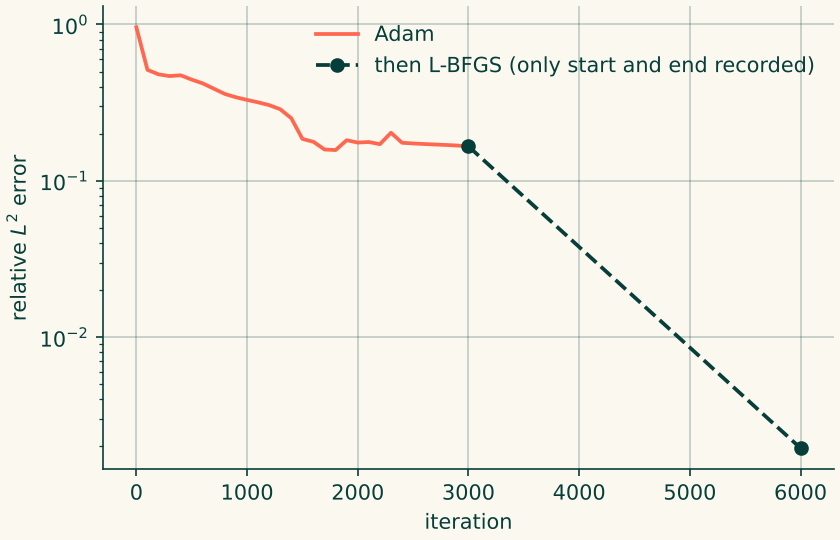
| Stage | Epoch / iteration | Total loss | Relative $L^2$ error |
|---|---|---|---|
| Adam | 0 | $4.5$ | $0.96$ |
| Adam | 500 | $3 \times 10^{-1}$ | $0.44$ |
| Adam | 1000 | $2 \times 10^{-1}$ | $0.33$ |
| Adam | 2000 | $4 \times 10^{-2}$ | $0.18$ |
| Adam | 3000 | $9 \times 10^{-3}$ | $0.17$ |
| then L-BFGS | 3000 more | $3 \times 10^{-5}$ | $\mathbf{2.0 \times 10^{-3}}$ |
Read the last two rows twice. After 3000 epochs of Adam the loss had fallen by a factor of 500 from where it started, yet the answer was still 17% wrong: the largest pointwise error was about 1.6 on a solution whose largest value is 1. The next 3000 iterations of L-BFGS took the error from 17% to 0.2%, a factor of about 85, and the largest pointwise error fell to $2.6\times10^{-2}$.
5. What it takes: a failed first attempt
The set-up above was reached by trying something smaller first. A first run used 4 hidden layers of 32 neurons, 6000 interior points, 6000 Adam epochs and only 500 L-BFGS iterations. It ended at a relative error of $7.6\times10^{-2}$, with the shock in about the right place but visibly smeared. Compared with that, the working set-up changed three things at once: a deeper network, more points, and many more L-BFGS iterations, so this experiment does not say which one mattered most. Treat the three as a package. If you want to find out which matters, vary them one at a time. That is a good exercise (see Section 7).
Lessons from the failure. (1) A loss that has dropped by orders of magnitude is not evidence of success, so always compare against a reference. (2) With a sharp feature, change the optimiser and the capacity before changing the loss weights. (3) Be ready to run longer: a shock takes patience.
6. If something goes wrong
| What you see | Likely cause | What to try |
|---|---|---|
| The loss falls but the answer is poor, with a smeared shock | Adam stalled; no second stage | Switch on L-BFGS as in Step 6 |
| The shock is smoother than the reference | Viscosity too large (0.01 instead of 0.01/pi), or a network that is too small |
Recheck the viscosity; try 8 × 20 |
| The picture is a mirror image | Missing minus sign in the initial condition | Re-enter -sin(pi*x) |
| The shock is in the wrong place | A mistake in the initial condition or the domain | Check $x\in[-1,1]$ and the initial condition |
L-BFGS ends immediately or the loss goes nan |
Starting L-BFGS from a poor point, or too large a step | Run more Adam epochs first, then L-BFGS |
| Error spread over the whole domain | Too few interior points | Raise to 10000 or more |
| Training takes far too long | L-BFGS with many points is slow | Use fewer L-BFGS iterations first, then add more |
7. Try it yourself
- Vary one thing at a time. Starting from the working set-up, change only the network (4 × 32), or only the point count (3000), or only the L-BFGS iterations (500). Which matters most? Record the error each time.
- Adam only. Skip L-BFGS and run Adam for 20000 epochs instead. How far does the error get?
- A larger viscosity. Set $\nu = 0.05$. The shock is much milder, so the problem is easier. How much smaller is the error, and does Adam alone now succeed?
- A smaller viscosity. Set $\nu = 0.001$. The shock is much sharper and the problem much harder. What happens to the error, and does the fix still work?
- Check the shock position. For this problem the shock stays at $x = 0$ for all time, by symmetry. Find, in your result, the $x$ at which the PINN crosses zero at $t=1$.
8. Recap
- Burgers' equation is nonlinear: the term $u\,u_x$ makes a smooth start develop a shock, and makes training much harder.
- When there is no formula, evaluate a reference numerically. Here, the Cole–Hopf transform gives an integral that a computer can compute. Check it against a second, independent method.
- A low loss is not a good answer. In the reference run Adam took the loss down by a factor of 500 and the answer was still 17% wrong.
- Use a two-stage optimiser: Adam to reach the right region, then L-BFGS to finish. Here it cut the error from 17% to 0.2%.
- Sharp features need capacity and points: a deeper network and many more collocation points than a smooth problem.
Next: back to a gentle problem on a curved domain, in Laplace's equation on a disc.
Reference script for the numbers quoted above: burgers_1d_reference.py, run as python burgers_1d_reference.py 3000 3000 8 20 10000. It contains the Cole–Hopf reference solution, is written by hand for checking this guide, and is not the Studio's generated output.