Poisson in one dimension
The smallest complete PINN: one unknown, one variable, no time, and an exact answer to grade it by. We build it in the Lab, run the script it writes, and look closely at how well it does.
This is the first worked example of the book. Everything in the chapters before this one appears in it once: a network, a loss made of residuals, derivatives by automatic differentiation, collocation points, an optimiser. The problem is chosen so that you can tell whether the result is right. It has an exact answer, and the network never sees it.
You do not need the Lab to follow the page, but it is built around one. The notebook is on this page as a file, and the Studio Tour explains every block it uses.
1. The problem
Find $u(x)$ on $0 < x < 1$ such that
$$ -\frac{d^2u}{dx^2} = \pi^2 \sin(\pi x), \qquad u(0) = 0, \qquad u(1) = 0 . $$
Read it as the steady temperature of a thin bar held at zero at both ends and heated along its length. The first equation is the governing equation; the other two are the boundary conditions. Together they single out one function.
The exact answer is easy to find. Try $u = \sin(\pi x)$: then $u'' = -\pi^2\sin(\pi x)$, so $-u'' = \pi^2\sin(\pi x)$, and $\sin 0 = \sin\pi = 0$. So
$$ u_{\text{exact}}(x) = \sin(\pi x). $$
The network will not be shown this. We keep it to grade the result.
The sign in the Lab
The Lab's Poisson block solves $\nabla^2 u = f$, with no minus sign. Our equation is $-u'' = \pi^2\sin(\pi x)$, which is $u'' = f$ with $f = -\pi^2\sin(\pi x)$. That is what you type into the block's source field. With the opposite sign you get the mirror image, $-\sin(\pi x)$, and a perfectly low loss.
2. How a PINN sees it
A PINN replaces the unknown function with a network $u_\theta(x)$ and asks it two questions, as in the residual as a loss. The method is that of Raissi, Perdikaris and Karniadakis (Raissi et al., 2019).
Is the equation satisfied inside? At collocation points $x_i$ in $(0,1)$ differentiate the network twice with automatic differentiation and form the residual, written the way the Lab writes it:
$$ r_\theta(x) = u_\theta''(x) - f(x), \qquad f(x) = -\pi^2\sin(\pi x). $$
Are the boundary conditions satisfied? At $x = 0$ and $x = 1$ the network should give zero.
The loss adds the mean square of each, with a weight:
$$ \mathcal{L}(\theta) = w_{\text{pde}}\,\frac{1}{N_r}\sum_{i=1}^{N_r} r_\theta(x_i)^2 \;+\; w_{1}\,u_\theta(0)^2 \;+\; w_{2}\,u_\theta(1)^2 . $$
Here all three weights are 1. In one dimension the boundary is two points, so this is enough; in two dimensions it is not.
Why tanh, not ReLU
The residual contains a second derivative of the network. A ReLU network is piecewise linear, so its second derivative is zero almost everywhere and the residual would say nothing. A smooth activation such as tanh has useful second derivatives. The Lab's default is tanh.
3. The same thing in the Lab
Each ingredient above is one block. The settings below are the Lab's defaults except the source term and the choice of equation.
| Block | Setting |
|---|---|
| Domain | Line, $x$ from 0 to 1, no time. 2000 interior points, 80 per boundary |
| PDE | Elliptic → Poisson, source -pi**2*sin(pi*x) |
| BC 1, BC 2 | Dirichlet, u = 0.0, on the left and right ends |
| Network | Hidden layers 40, 40, 40, 40, tanh, Xavier initialisation (5,041 parameters) |
| Loss | Mean square, PDE weight 1, BC weights [1, 1] |
| Optimiser | Adam, learning rate 0.001, 5000 epochs |
| Train | Seed 0, checkpoint model.pt |
| Visualisation, Report | Defaults |
You can build it by hand by following Build a notebook from an empty canvas, or open the finished notebook: download poisson-1d.omega-notebook.json, go to the Lab and choose Open a notebook file….
The script the Lab writes for it is poisson_1d.py. It is exactly what the Generate code button gives. Its heart, the residual, is this:
# not run
def residual_pde1(pts):
    u = field(pts, 0)
    x = pts[:, 0:1]
    g1 = grad_of(u, pts)
    u_x = g1[:, 0:1]
    g2_x = grad_of(u_x, pts)
    u_xx = g2_x[:, 0:1]
    f = ((-(math.pi ** 2.0)) * torch.sin((math.pi * x)))
    return (u_xx) - f
and the same program, written out by hand in about twenty lines, is below. It uses the same network (four layers of 40, tanh, Xavier weights, inputs scaled to $[-1, 1]$), the same loss, the same optimiser and the same number of epochs. Run it to see the whole method at once.
import math, torch

torch.manual_seed(0)
layers = []
for n_in, n_out in [(1, 40), (40, 40), (40, 40), (40, 40)]:
    layers += [torch.nn.Linear(n_in, n_out), torch.nn.Tanh()]
net = torch.nn.Sequential(*layers, torch.nn.Linear(40, 1))
for m in net:
    if isinstance(m, torch.nn.Linear):
        torch.nn.init.xavier_normal_(m.weight)
        torch.nn.init.zeros_(m.bias)

u = lambda x: net(2 * x - 1)                       # scale [0, 1] to [-1, 1]

def residual(x):                                    # u'' - f, with f = -pi^2 sin(pi x)
    ux, = torch.autograd.grad(u(x).sum(), x, create_graph=True)
    uxx, = torch.autograd.grad(ux.sum(), x, create_graph=True)
    return uxx + math.pi ** 2 * torch.sin(math.pi * x)

x_in = torch.rand(2000, 1).requires_grad_(True)     # collocation points
x_b = torch.tensor([[0.0], [1.0]])                  # the two boundary points
opt = torch.optim.Adam(net.parameters(), lr=1e-3)

for epoch in range(5000):
    opt.zero_grad()
    loss = residual(x_in).pow(2).mean() + u(x_b).pow(2).sum()
    loss.backward()
    opt.step()

x = torch.linspace(0, 1, 1001).reshape(-1, 1)
with torch.no_grad():
    err = u(x) - torch.sin(math.pi * x)
print(f"final loss {loss.item():.2e}   relative L2 error {(err.norm() / torch.sin(math.pi * x).norm()).item():.1e}")
final loss 1.71e-06 relative L2 error 1.0e-04
Do not compare its digits with the Lab runs in the next section. It draws its random numbers differently (it uses the two boundary points directly, where the Lab draws 80 copies of each), so it is one more sample from the same family of runs, not a reproduction of one. What it shows is that the method is this short.
The residual function is the whole idea in four lines: the first autograd.grad differentiates the network once, the second differentiates the result again, and create_graph=True keeps those derivatives themselves differentiable so that the optimiser can later push the residual down.
4. The result
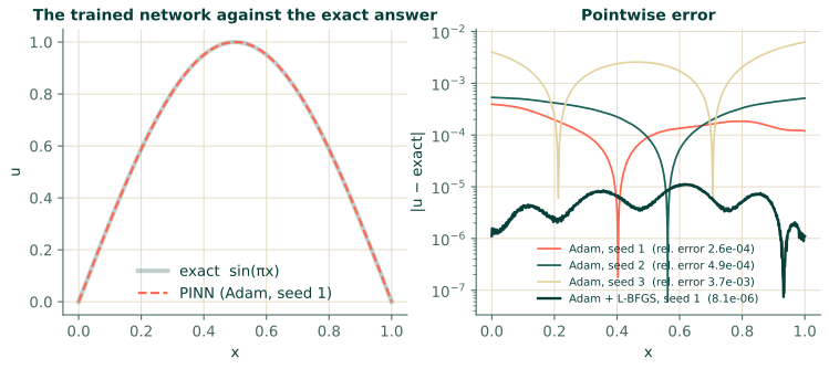
We ran the Lab's script six times, changing nothing but the seed that sets the starting weights: three times with Adam alone, and three times with the optimiser's Second stage ticked (Adam for 5000 epochs, then L-BFGS for up to 500 iterations). The error is the relative $L^2$ error against $\sin(\pi x)$ on 1001 evenly spaced points, which are not the points the network trained on.
| Run | Relative $L^2$ error | Loss at the end | Lowest loss seen |
|---|---|---|---|
| Adam, seed 1 | $2.6\times10^{-4}$ | $6.1\times10^{-5}$ | $3.4\times10^{-5}$ |
| Adam, seed 2 | $4.9\times10^{-4}$ | $1.1\times10^{-5}$ | $7.5\times10^{-6}$ |
| Adam, seed 3 | $3.7\times10^{-3}$ | $2.9\times10^{-3}$ | $9.6\times10^{-6}$ |
| Adam + L-BFGS, seed 1 | $8.1\times10^{-6}$ | $2.3\times10^{-6}$ | $2.3\times10^{-6}$ |
| Adam + L-BFGS, seed 2 | $5.9\times10^{-6}$ | $1.6\times10^{-6}$ | $1.6\times10^{-6}$ |
| Adam + L-BFGS, seed 3 | $1.3\times10^{-5}$ | $9.4\times10^{-6}$ | $9.4\times10^{-6}$ |
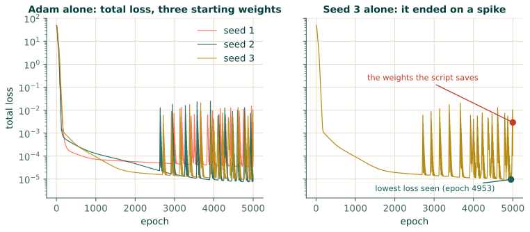
The total loss started near 50 in every run (the untrained network satisfies neither the equation nor the boundary conditions) and fell to about $10^{-3}$ within the first 200 epochs. Each run took about 40 seconds on the two-core cloud machine we used; yours will differ. These numbers are repeatable on one machine and will shift a little on another.
5. Why the last run is not like the others
Look at the table's third row. Seed 3 is the worst of the Adam runs by a factor of ten, yet at some point in training its loss was as low as any other run's: $9.6\times10^{-6}$, at epoch 4953. It ended at $2.9\times10^{-3}$.
The cause is in the right-hand panel of Figure 13.2. From about epoch 2700 on, Adam's loss on this problem is not a smooth descent. It is a descent punctuated by spikes, in which the loss jumps up by one to two orders of magnitude and recovers within a few epochs. All three Adam runs do it. In seed 3 the last epoch landed on one, and the script saves the weights from the last epoch, not from the best. That is a fact about the script, not about PINNs: it keeps the network it ends with.
There are three ways to handle it, in increasing order of effort. Run more than once and report the spread, as the table does. Finish with L-BFGS, which does not spike and, as the lower rows show, lowered the error by a factor of 30 to 300 here. Or edit the script to remember the best weights as it goes, which is a few lines in the training loop. Whichever you choose, do not judge a PINN by a single run.
6. Exercises
Each changes one block and has an exact answer to grade against. Remember the Lab's sign: if the book's equation is $-u'' = g$, enter $f = -g$.
- A different source. Take $-u'' = 1$ with the same ends. What is the exact solution, and what do you enter as the source?
- A non-zero end. Keep $-u'' = \pi^2\sin(\pi x)$ but ask for $u(1) = 1$. What is the exact solution, and which block changes?
- Fewer points. Cut the interior points to 10. Measure the error on a fine grid that is not the training points. What do you see between them?
- A smaller network. Try one hidden layer of 8 neurons. At what width does the error stop improving?
Answers to 1 and 2
- Integrating twice gives $u = \tfrac12 x(1-x)$, which is zero at both ends and has $-u'' = 1$. In the Lab, $-u'' = 1$ means $u'' = -1$, so the source $f$ is
-1. - $u = \sin(\pi x) + x$. It has $-u'' = \pi^2\sin(\pi x)$ because $x$ is linear, and $u(0) = 0$, $u(1) = 1$. Only BC 2 changes: its
u =field becomes1.0.
Exercises 3 and 4 have no single right answer; they are to be run. Judge each by the relative error on a separate grid, over several seeds.
7. Recap
- A PINN trains a network to make the residual of the equation and the boundary error small together, with derivatives from automatic differentiation.
- In the Lab each part is one block, and the script it writes is plain PyTorch you can read, as the hand-written version above shows.
- Even for the easiest problem, runs differ. Report several, and say how the weights at the end of the run were chosen.
- Adam alone is noisy; adding an L-BFGS stage gave a much lower and steadier error here.
Next: the same problem on a square, where the boundary weights stop being optional. Poisson on a square.
References
- Raissi, M., Perdikaris, P., & Karniadakis, G. E. (2019). Physics-informed neural networks: A deep learning framework for solving forward and inverse problems involving nonlinear partial differential equations. Journal of Computational Physics, 378, 686–707. doi:10.1016/j.jcp.2018.10.045