Scientific ML Studio

The mean squared error is an average over all $N$ data points: $\mathcal{L}(\theta) = \frac1N\sum_{i=1}^{N}\ell_i(\theta)$, where $\ell_i$ is the squared residual at point $i$. Its gradient is the average of the individual gradients,

$$\nabla\mathcal{L}(\theta) = \frac{1}{N}\sum_{i=1}^{N}\nabla\ell_i(\theta).$$

Computing that means looking at every point, at every step. For a data set of a million images that is wasteful: nearly all the points carry nearly the same information about which way is downhill.

Mini-batches

The remedy is to use only a random subset, a mini-batch $B$ of $m$ points, and estimate

$$\nabla\mathcal{L}(\theta) \approx g_B(\theta) = \frac{1}{m}\sum_{i\in B}\nabla\ell_i(\theta).$$

The estimate is unbiased: averaged over all possible random batches it equals the true gradient. Each individual estimate is noisy, with a spread that shrinks like $1/\sqrt{m}$. Take the 1,000-point line fit from Section 3.2, and measure how much the gradient jumps around at its optimum, where the exact gradient is zero:

import numpy as np

rng = np.random.default_rng(0)
N = 1000
x = rng.uniform(-1, 1, N)
y = 3 * x + 1 + 0.3 * rng.normal(size=N)
X = np.column_stack([x, np.ones(N)])
theta_star = np.linalg.lstsq(X, y, rcond=None)[0]

def batch_grad(theta, idx):
    Xb = X[idx]
    return 2 / len(idx) * Xb.T @ (Xb @ theta - y[idx])

rng = np.random.default_rng(2)
print(" batch size   spread of gradient (std of components)")
for m in [10, 100, 1000]:
    grads = np.array([batch_grad(theta_star, rng.choice(N, m, replace=False)) for _ in range(500)])
    print(f"{m:8d}      {grads.std(axis=0).round(3)}")

 batch size   spread of gradient (std of components)
      10      [0.111 0.194]
     100      [0.032 0.058]
    1000      [0. 0.]

At the optimum the true gradient is zero, yet a batch of ten reports a gradient of order $0.1$ to $0.2$: pure noise from sampling. A batch of 100 is about three times quieter ($\sqrt{10}\approx 3.2$), and the batch of all 1,000 points has no noise at all. This is stochastic gradient descent (SGD) when $m = 1$, mini-batch SGD for $1 < m < N$, and plain full-batch gradient descent for $m = N$.

Does the noisy version still work?

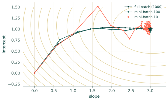
Run the same line fit with mini-batches of 10 and 100, the same step size $\eta = 0.3$ and the same 200 steps as before:

for m in [10, 100]:
    rng = np.random.default_rng(1)
    theta = np.zeros(2)
    for _ in range(200):
        theta = theta - 0.3 * batch_grad(theta, rng.choice(N, m, replace=False))
    err = np.linalg.norm(theta - theta_star)
    print(f"batch {m:4d}:  theta = {theta.round(3)}   distance from optimum = {err:.3f}")
print("exact optimum :", theta_star.round(3))

batch   10:  theta = [2.954 0.879]   distance from optimum = 0.125
batch  100:  theta = [2.989 0.999]   distance from optimum = 0.009
exact optimum : [2.997 0.997]

Both runs head to the right place. The small batch ends a noticeable distance away and keeps jittering around the optimum instead of settling on it, because it is always acting on a noisy slope. Two standard cures are to shrink $\eta$ over time (a learning-rate schedule, see Chapter 9) and to use a larger batch late in training.

Contours of a bowl with a smooth path for full-batch descent and a jittery path for mini-batch descent, both ending near the minimum. — **Figure 3.4.** Full-batch descent takes a smooth path; mini-batch descent follows a noisier one, with the noise growing as the batch shrinks.

Epochs

One pass in which every data point has been used once is an epoch. With $N = 1000$ and $m = 100$ one epoch is 10 steps. Counting in epochs lets you compare runs with different batch sizes on equal terms.

Where this goes in a PINN

A PINN has no data set in the usual sense, but it has the same structure. The residual loss is an average over collocation points, $\frac1M\sum_j r(\mathbf{x}_j)^2$, so it can be estimated from a random subset of them. Two strategies are common: use a fixed set of points and the whole of it at each step (full batch), or draw fresh random points at each step (mini-batch, with the added benefit that the network sees new places every time). Chapter 7 compares them. Many PINN workflows also finish with a full-batch optimiser, which needs the exact gradient; Chapter 9 explains why.

Exercises

A data set has $N = 2400$ points and you use a batch of $m = 64$. How many steps make one epoch (round up)?
By what factor does the standard deviation of the gradient fall when you go from $m = 25$ to $m = 400$?
Why does an unbiased but noisy gradient still lead to the minimum, on average?

Answers

$2400/64 = 37.5$, so 38 steps.
$\sqrt{400/25} = 4$ times smaller.
Because in expectation each step moves exactly as the true gradient would. The noise adds jitter around the intended path, and shrinking it (small $\eta$, larger batches) reduces the jitter.

Recap

A mini-batch gradient is an unbiased, noisy estimate of the full gradient, with noise falling like $1/\sqrt{m}$.
It works because it costs much less per step; it leaves jitter near the optimum, reduced by smaller steps or larger batches.
A PINN's residual loss is also an average, so it too can be estimated from random subsets of collocation points.