Gradient descent, step by step
Take a small step against the gradient, repeat. The whole algorithm is one line, and its behaviour is governed by one number: the learning rate.
Section 3.1 established that $-\nabla\mathcal{L}$ points downhill. Gradient descent takes the obvious step:
$$\theta_{k+1} = \theta_k - \eta\,\nabla\mathcal{L}(\theta_k).$$
The number $\eta > 0$ is the learning rate (or step size). Start from some $\theta_0$, apply the rule over and over, and, if all goes well, $\theta_k$ settles near a minimum. In code it is very short:
import numpy as np

def gradient_descent(grad, theta0, eta, steps):
    theta = np.array(theta0, dtype=float)
    path = [theta.copy()]
    for _ in range(steps):
        theta = theta - eta * grad(theta)
        path.append(theta.copy())
    return np.array(path)
Everything interesting about training is in the choice of $\eta$ and in the shape of the landscape.
One parameter: what the learning rate does
Take the simplest possible loss, $\mathcal{L}(\theta) = \tfrac{a}{2}\theta^2$, with slope $a\theta$. One step gives
$$\theta_{k+1} = \theta_k - \eta a\theta_k = (1 - \eta a)\,\theta_k, \qquad\text{so}\qquad \theta_k = (1 - \eta a)^k\,\theta_0.$$
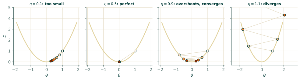
The distance to the minimum is multiplied by the same factor, $1 - \eta a$, at every step. That gives four regimes:
| $\eta a$ | factor $1-\eta a$ | behaviour |
|---|---|---|
| between 0 and 1 | between 0 and 1 | steady, one-sided convergence |
| exactly 1 | 0 | lands on the minimum in one step |
| between 1 and 2 | between $-1$ and 0 | overshoots every step, but still converges |
| above 2 | below $-1$ | each overshoot is bigger than the last: it diverges |
Convergence therefore requires $0 < \eta < 2/a$. Try it with $a = 2$, where the limit is $\eta < 1$:
a = 2.0
grad_1d = lambda th: a * th

for eta in [0.1, 0.5, 0.9, 1.1]:
    path = gradient_descent(grad_1d, [1.0], eta, steps=6)[:, 0]
    print(f"eta = {eta:3.1f}  factor = {1 - eta * a:+.1f}  theta_k =", np.round(path, 3))
eta = 0.1  factor = +0.8  theta_k = [1.    0.8   0.64  0.512 0.41  0.328 0.262]
eta = 0.5  factor = +0.0  theta_k = [1. 0. 0. 0. 0. 0. 0.]
eta = 0.9  factor = -0.8  theta_k = [ 1.    -0.8    0.64  -0.512  0.41  -0.328  0.262]
eta = 1.1  factor = -1.2  theta_k = [ 1.    -1.2    1.44  -1.728  2.074 -2.488  2.986]
Read each line against the table. Too small a step crawls; $\eta = 0.5$ hits the minimum immediately; $0.9$ bounces from side to side while shrinking; $1.1$ is beyond the limit and grows.
Two parameters: the stretched bowl
Now return to $\mathcal{L}(\theta) = \tfrac12(\theta_1^2 + 25\theta_2^2)$. The two directions have different curvature, $a_1 = 1$ and $a_2 = 25$, and the same $\eta$ must serve both. Each coordinate follows the 1D rule with its own factor: $(1 - \eta)^k$ for $\theta_1$ and $(1 - 25\eta)^k$ for $\theta_2$.
The steep direction sets the limit, $\eta < 2/25 = 0.08$, or $\theta_2$ blows up. But with $\eta$ that small, the gentle direction contracts by only $1 - \eta$ per step. Watch:
grad_2d = lambda t: np.array([t[0], 25 * t[1]])
start = [5.0, 1.0]

for eta in [0.01, 0.04, 0.07, 0.09]:
    path = gradient_descent(grad_2d, start, eta, steps=100)
    th1, th2 = path[-1]
    print(f"eta = {eta:.2f}   after 100 steps:  theta_1 = {th1:9.4f}   theta_2 = {th2:9.4f}")
eta = 0.01   after 100 steps:  theta_1 =    1.8302   theta_2 =    0.0000
eta = 0.04   after 100 steps:  theta_1 =    0.0844   theta_2 =    0.0000
eta = 0.07   after 100 steps:  theta_1 =    0.0035   theta_2 =    0.0000
eta = 0.09   after 100 steps:  theta_1 =    0.0004   theta_2 = 4909093465.2977
With $\eta = 0.07$ the steep coordinate has been driven to zero (its factor is $-0.75$, so it flips sign as it shrinks), while $\theta_1$, the gentle one, is still crawling: its factor is only $0.93$ per step. Pushing $\eta$ past $0.08$ makes $\theta_2$ explode. You cannot fix one without breaking the other.
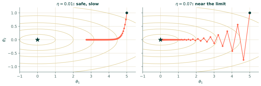
The ratio of the largest to the smallest curvature, here $25/1 = 25$, is the condition number of the problem. The larger it is, the worse gradient descent behaves, and this is the technical meaning of "ill-conditioned" that appeared in the exercise to Section 1.2. A PDE residual loss is typically very ill-conditioned, because the derivative operators inside it stretch some directions of parameter space by orders of magnitude more than others. That is why the better optimisers of Section 3.5 and Chapter 9 matter.
Checking against the closed form
Gradient descent should find the same answer as the normal equations of Section 1.2, when both apply. Fit a line $y \approx \theta_1 x + \theta_2$ to 1,000 noisy points:
rng = np.random.default_rng(0)
N = 1000
x = rng.uniform(-1, 1, N)
y = 3 * x + 1 + 0.3 * rng.normal(size=N)
X = np.column_stack([x, np.ones(N)])

closed_form = np.linalg.lstsq(X, y, rcond=None)[0]

grad_mse = lambda th: 2 / N * X.T @ (X @ th - y)
path = gradient_descent(grad_mse, [0.0, 0.0], eta=0.3, steps=200)

print("normal equations :", np.round(closed_form, 5))
print("gradient descent :", np.round(path[-1], 5))
print("loss at start/end:", round(float(np.mean((X @ path[0] - y) ** 2)), 4),
      round(float(np.mean((X @ path[-1] - y) ** 2)), 4))
normal equations : [2.99689 0.99651]
gradient descent : [2.99689 0.99651]
loss at start/end: 4.2095 0.0946
The two answers agree to five decimals: the loop found the bottom of the bowl without being told where it was.
When to stop
Gradient descent never arrives; it only gets closer. Practical stopping rules are a fixed number of steps (the usual choice), a gradient whose norm is below a tolerance, a loss that has stopped changing, or a validation error that has started to rise (Section 1.3). In PINN work the loss curve is watched closely, as Chapter 12 explains, because a loss that stops falling is not necessarily a solution.
Exercises
- For $\mathcal{L} = \tfrac{a}{2}\theta^2$ with $a = 10$, what is the largest stable learning rate? What does $\eta = 0.1$ do?
- For $\mathcal{L} = \tfrac12(\theta_1^2 + 100\theta_2^2)$, what is the condition number and the largest stable $\eta$?
- Using the largest safe $\eta$ you found, roughly how many steps does it take for $\theta_1$ to shrink by a factor of $10^{3}$?
Answers
- $\eta < 2/10 = 0.2$. At $\eta = 0.1$, $\eta a = 1$: the factor is 0, so it lands on the minimum in one step.
- Condition number $100/1 = 100$; stability needs $\eta < 2/100 = 0.02$.
- The factor for $\theta_1$ is $1 - \eta \approx 0.98$. We need $0.98^k = 10^{-3}$, so $k = \ln(10^{-3})/\ln(0.98) \approx 342$ steps. Ill-conditioning makes a "simple" problem take hundreds of steps.
Recap
- Gradient descent: $\theta \leftarrow \theta - \eta\nabla\mathcal{L}$. It converges only if $\eta < 2/a$ for the stiffest direction.
- In a stretched landscape the stiff direction caps $\eta$ and the soft direction then crawls. The ratio is the condition number.
- Agreement with a closed form (when one exists) is a good test that your implementation is correct.