Scientific ML Studio

Section 3.2 ended with a complaint: in a stretched valley the learning rate is capped by the steep direction, and progress along the shallow one is slow. Two ideas, both a few lines of code, attack this.

Momentum

Picture a ball rolling on the loss surface instead of a point that teleports downhill. It has inertia: it keeps some of its previous velocity. Keep a running velocity $\mathbf{v}$ that blends the old velocity with the new gradient:

$$\mathbf{v}_{k+1} = \beta\,\mathbf{v}_k + \nabla\mathcal{L}(\theta_k),\qquad \theta_{k+1} = \theta_k - \eta\,\mathbf{v}_{k+1}.$$

The momentum coefficient $\beta$ (typically $0.9$) says how much of the past to keep. Across the valley, where the gradient flips sign every step, the contributions cancel in $\mathbf{v}$ and the zigzag is damped. Along the valley, where the gradient keeps the same sign, they accumulate, and the effective step grows up to $1/(1-\beta)$ times larger (ten times for $\beta = 0.9$). Both effects help.

Adam

Momentum fixes the direction. Adam also fixes the scale, separately for each parameter. It keeps two running averages of the gradient $\mathbf{g}$, the mean and the mean of its square:

$$ \begin{aligned} \mathbf{m}_k &= \beta_1\mathbf{m}_{k-1} + (1-\beta_1)\,\mathbf{g}_k, & \mathbf{s}_k &= \beta_2\mathbf{s}_{k-1} + (1-\beta_2)\,\mathbf{g}_k^{2},\\[2pt] \hat{\mathbf{m}}_k &= \frac{\mathbf{m}_k}{1-\beta_1^{\,k}}, & \hat{\mathbf{s}}_k &= \frac{\mathbf{s}_k}{1-\beta_2^{\,k}}, \end{aligned} \qquad \theta_{k+1} = \theta_k - \eta\,\frac{\hat{\mathbf{m}}_k}{\sqrt{\hat{\mathbf{s}}_k} + \varepsilon}. $$

The squares and the square root are element-wise. The division by $\sqrt{\hat{\mathbf{s}}_k}$ is the key: a parameter whose gradients are always large gets its step scaled down, one whose gradients are tiny gets scaled up, so every parameter moves at a comparable rate. The hats undo the bias from starting the averages at zero. The method is due to Kingma & Ba (2014), who suggest $\beta_1 = 0.9$, $\beta_2 = 0.999$, $\varepsilon = 10^{-8}$; those are also PyTorch's defaults. In practice only the learning rate $\eta$ is usually tuned.

Comparing them honestly

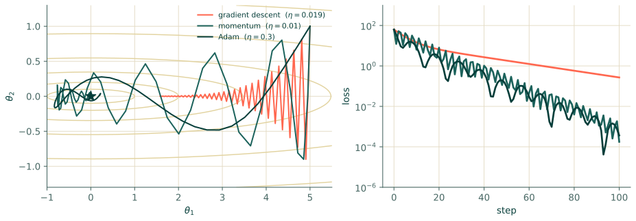
An optimiser comparison with one hand-picked learning rate proves little. Here we give each method a range of rates on a stretched bowl with curvatures $1$ and $100$ (condition number 100), run 100 steps from the same start, and print the final loss for each.

import numpy as np

H = np.array([1.0, 100.0])                 # curvatures; L = 0.5 * sum(H * theta^2)
loss = lambda t: 0.5 * np.sum(H * t ** 2)
grad = lambda t: H * t
start = np.array([5.0, 1.0])

def run_gd(eta, steps=100):
    t = start.copy()
    for _ in range(steps):
        t = t - eta * grad(t)
    return loss(t)

def run_momentum(eta, beta=0.9, steps=100):
    t, v = start.copy(), np.zeros(2)
    for _ in range(steps):
        v = beta * v + grad(t)
        t = t - eta * v
    return loss(t)

def adam_path(lr, steps=100, b1=0.9, b2=0.999, eps=1e-8):
    t, m, s = start.copy(), np.zeros(2), np.zeros(2)
    for k in range(1, steps + 1):
        g = grad(t)
        m = b1 * m + (1 - b1) * g
        s = b2 * s + (1 - b2) * g * g
        t = t - lr * (m / (1 - b1 ** k)) / (np.sqrt(s / (1 - b2 ** k)) + eps)
    return t

run_adam = lambda lr, steps=100: loss(adam_path(lr, steps))

def table(name, fn, rates):
    print(f"{name:9s}" + "".join(f"{r:>10g}" for r in rates))
    print(f"{'  loss':9s}" + "".join(f"{fn(r):10.1e}" for r in rates))

table("GD  eta", run_gd, [0.001, 0.003, 0.01, 0.019, 0.03])
table("Mom eta", run_momentum, [0.0005, 0.001, 0.003, 0.01, 0.019])
table("Adam lr", run_adam, [0.01, 0.03, 0.1, 0.3, 1.0])

GD  eta       0.001     0.003      0.01     0.019      0.03
  loss      1.0e+01   6.9e+00   1.7e+00   2.7e-01   8.0e+61
Mom eta      0.0005     0.001     0.003      0.01     0.019
  loss      4.8e+00   1.7e+00   2.5e-03   1.8e-04   1.7e-03
Adam lr        0.01      0.03       0.1       0.3         1
  loss      1.1e+01   2.8e+00   1.2e-03   3.7e-04   3.6e-04

Three things to read off. Plain GD has a cliff: its best rate (0.019, just below the limit $2/100 = 0.02$) leaves a loss of about $0.3$ after 100 steps, and one notch higher it diverges to $10^{61}$. Momentum reaches about $10^{-4}$ with the right rate, over a thousand times better, using the same gradients. Adam reaches a similar level, and, importantly, it does so over a wide range of rates ($0.1$ to $1$) with no cliff. That forgiveness is why Adam is a common first choice for training networks, PINNs included, where we rarely know the right scale in advance.

Left: paths of gradient descent, momentum and Adam on a narrow valley. Gradient descent zigzags tightly across the valley and creeps along it; momentum and Adam swing wider but cover much more distance along the valley. Right: loss against step on a log scale; gradient descent falls slowly and steadily, momentum and Adam fall much faster with visible wobbles. — **Figure 3.6.** The three optimisers on the same bowl, each with its best rate from the table. Left: the first 60 steps in parameter space. Gradient descent is boxed in by the stability limit; momentum and Adam swing wider but travel much further along the valley. Right: loss against step for all 100 steps.

A caveat on this experiment

Here the valley's axes line up with the coordinates, which is the case where Adam's per-parameter scaling is ideal. In a real network the stiff directions are mixtures of many weights, and Adam helps less cleanly. It is still a very good default. Chapter 9 goes into where it stalls and why PINNs often switch to a second-order method such as L-BFGS to finish.

Using it in PyTorch

You will not write these loops yourself: torch.optim.SGD(params, lr, momentum=0.9) and torch.optim.Adam(params, lr) do. To make sure we have understood the formulas and not merely typed them in, run PyTorch's Adam next to our version on the same problem and compare the final parameters:

import torch

theta = torch.tensor(start, requires_grad=True)
curv = torch.tensor(H)
opt = torch.optim.Adam([theta], lr=0.3)
for _ in range(100):
    opt.zero_grad()
    l = 0.5 * (curv * theta ** 2).sum()
    l.backward()
    opt.step()

print("PyTorch Adam:", theta.detach().numpy().round(6))
print("our Adam    :", adam_path(0.3).round(6))
print("max difference:", float(np.abs(theta.detach().numpy() - adam_path(0.3)).max()))

PyTorch Adam: [ 0.021548 -0.001642]
our Adam    : [ 0.021548 -0.001642]
max difference: 6.5052130349130266e-18

They agree to many decimal places, so the formulas above are exactly what the library computes.

Exercises

With $\beta = 0.9$, momentum on a gradient that is constant, $g$, converges to a velocity of $10g$. Verify using $v = \beta v + g$ at the fixed point.
Adam's update has size about $\eta$ per parameter no matter how large the gradient is (as long as it is steady). Why does that help when the gradient of one weight is $10^{-4}$ and another's is $10^{2}$?
After one Adam step from $m_0 = s_0 = 0$ with gradient $g$, what is the update (ignore $\varepsilon$)? (Hint: work out $\hat m_1$ and $\hat s_1$.)

Answers

Fixed point: $v = \beta v + g \Rightarrow v(1-\beta) = g \Rightarrow v = g/(1-\beta) = 10g$.
Plain gradient descent would move the second weight a million times more than the first. Adam normalises by the gradient's typical size, so both move on the same scale and one learning rate suits both.
$m_1 = (1-\beta_1)g$ so $\hat m_1 = g$; $s_1 = (1-\beta_2)g^2$ so $\hat s_1 = g^2$. The update is $\eta\, g/|g| = \eta\,\mathrm{sign}(g)$: the first step has size exactly $\eta$ in every coordinate.

Recap

Momentum smooths the direction by keeping a running velocity; Adam additionally rescales each parameter by its recent gradient size.
Adam is forgiving about its learning rate, which makes it the standard first optimiser, including for PINNs.
Always compare optimisers over a range of rates, and check your own implementation against the library's.

Momentum and Adam

References

- Kingma, D. P., & Ba, J. (2014). Adam: A method for stochastic optimization. arXiv preprint. arXiv:1412.6980