Layers and the forward pass

One neuron is a weak model. A layer is a row of neurons that all look at the same inputs, each with its own weights and bias. A network is a stack of layers, each reading the outputs of the one before. This arrangement is called a multilayer perceptron (MLP) or fully connected network, and it is the network used in almost every PINN.

One layer, in matrix form

Let a layer have $n_\text{in}$ inputs and $n_\text{out}$ neurons. Collect the weights of all its neurons in a matrix $W$ with one row per neuron, so $W$ has shape $(n_\text{out}, n_\text{in})$, and the biases in a vector $\mathbf{b}$ of length $n_\text{out}$. The whole layer is then

$$\mathbf{a} = \sigma\bigl(W\mathbf{x} + \mathbf{b}\bigr),$$

with $\sigma$ applied to each entry separately. A matrix–vector product does all the weighted sums at once.

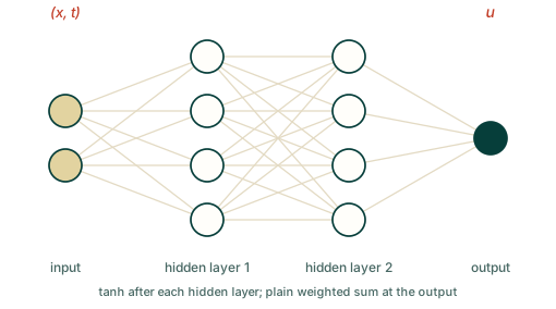
A full network with two hidden layers and a scalar output is

$$ \begin{aligned} \mathbf{h}_1 &= \sigma\bigl(W_1\mathbf{x} + \mathbf{b}_1\bigr),\\ \mathbf{h}_2 &= \sigma\bigl(W_2\mathbf{h}_1 + \mathbf{b}_2\bigr),\\ f_\theta(\mathbf{x}) &= W_3\mathbf{h}_2 + \mathbf{b}_3. \end{aligned} $$

Two things to notice. The layers between input and output are called hidden layers, because we never observe their values directly. And the last layer has no activation: for regression the output should be free to take any value, positive or negative and of any size, so we leave it as a plain weighted sum.

Counting parameters

A layer from $n_\text{in}$ to $n_\text{out}$ has $n_\text{out}\,n_\text{in}$ weights and $n_\text{out}$ biases:

$$\#\text{params} = n_\text{out}\,(n_\text{in} + 1).$$

For the 2–4–4–1 network of Figure 2.3: $4(2+1) + 4(4+1) + 1(4+1) = 12 + 20 + 5 = 37$. A typical PINN network, 2–50–50–50–50–1, already has 7,851 parameters. They are the unknowns of the optimisation.

The forward pass in NumPy

Running an input through the network to get an output is the forward pass. Here it is in plain NumPy, for a network whose layer sizes are given as a list:

import numpy as np

def init(sizes, seed=0):
    """Random weights; the scale 1/sqrt(fan_in) keeps the signals from blowing up or dying."""
    rng = np.random.default_rng(seed)
    params = []
    for n_in, n_out in zip(sizes[:-1], sizes[1:]):
        W = rng.normal(size=(n_out, n_in)) / np.sqrt(n_in)
        b = np.zeros(n_out)
        params.append((W, b))
    return params

def forward(params, x):
    """x has shape (n_in,) for one point or (N, n_in) for N points."""
    h = np.atleast_2d(x)
    for W, b in params[:-1]:
        h = np.tanh(h @ W.T + b)          # hidden layers: bend
    W, b = params[-1]
    return h @ W.T + b                     # last layer: plain weighted sum

params = init([2, 4, 4, 1])
print("shapes of W:", [W.shape for W, _ in params])
print("parameters :", sum(W.size + b.size for W, b in params))

points = np.array([[0.0, 0.0], [0.5, 0.5], [1.0, 0.0]])
print("outputs    :", np.round(forward(params, points).ravel(), 4))

shapes of W: [(4, 2), (4, 4), (1, 4)]
parameters : 37
outputs    : [ 0.     -0.314  -0.3883]

The parameter count agrees with the hand count. Two details in the code are worth a note.

Rows are points. We store a batch of $N$ points as an array of shape $(N, n_\text{in})$, so the layer computes h @ W.T + b: the transpose of the formula above, which is the convention every deep-learning library uses. It lets one call process thousands of points at once, which is how a PINN evaluates all its collocation points together.

The initial scale. Weights are started at random, and the scale matters. If they are too large the signals grow layer by layer; too small and they shrink to nothing. Dividing by $\sqrt{n_\text{in}}$ is a simple rule in the spirit of the initialisation schemes of Glorot & Bengio (2010), who studied exactly why deep feedforward networks were hard to train from a poor start. PyTorch has built-in initialisers (Section 2.5), so you will not write this yourself.

Why depth needs the bend

Section 2.1 said that without the activation a stack of neurons collapses to one linear map. We can check it:

rng = np.random.default_rng(1)
W1, W2 = rng.normal(size=(5, 3)), rng.normal(size=(2, 5))
x = rng.normal(size=3)

two_layers = W2 @ (W1 @ x)           # two linear layers, no activation
one_layer = (W2 @ W1) @ x            # a single matrix, W = W2 W1
print("same output:", np.allclose(two_layers, one_layer))

same output: True

Matrix multiplication is associative, so any number of linear layers equals one. Only the activations between them make a deeper network more expressive than a shallower one.

Width and depth

Two numbers describe the shape of an MLP: its width (neurons per hidden layer) and its depth (number of hidden layers). Worked PINN examples typically use a few hidden layers of tens of neurons each. There is no formula for the best choice; Part 4 returns to it as a design question.

Exercises

1. How many parameters does a 3–10–10–2 network have?
2. What are the shapes of $W_1$, $W_2$, $W_3$ for the network in the previous question?
3. A student removes all activations from a 5-layer network. What function class does it now represent?

Recap

• A layer is $\sigma(W\mathbf{x} + \mathbf{b})$; a network is a stack of layers with a plain linear last layer.
• A layer from $n_\text{in}$ to $n_\text{out}$ has $n_\text{out}(n_\text{in}+1)$ parameters.
• Points are stored as rows, and the forward pass is a few matrix multiplications that handle a whole batch at once.

References

- Glorot, X., & Bengio, Y. (2010). Understanding the difficulty of training deep feedforward neural networks. Proceedings of Machine Learning Research, 9, 249–256. https://proceedings.mlr.press/v9/glorot10a.html