Loss functions: a number that says how wrong

To choose $\theta$ we need a way to compare two candidate parameter vectors and say which is better. Humans do that by eye; a computer needs a number. That number is the loss (or cost, or objective), written $\mathcal{L}(\theta)$. Training is then a search for the $\theta$ that makes it small.

Residuals and the mean squared error

The basic ingredient is the residual at one data point, the gap between what the model says and what was measured:

$$r_i(\theta) = f_\theta(x_i) - y_i.$$

A single number for the whole data set is the mean squared error (MSE):

$$\mathcal{L}(\theta) = \frac{1}{N}\sum_{i=1}^{N} r_i(\theta)^2 = \frac{1}{N}\sum_{i=1}^{N}\bigl(f_\theta(x_i) - y_i\bigr)^2.$$

Why square the residuals rather than add them up? Three reasons, in increasing order of importance:

1. Signs would cancel: a model that is $+1$ off at one point and $-1$ off at another would score zero.
2. Big mistakes cost more than small ones, which usually matches what we care about.
3. The result is a smooth function of $\theta$. The derivative of $r^2$ is $2r\,r'$, defined everywhere, so we can follow the slope downhill. This is the property training relies on in Chapter 3.

A loss you can see

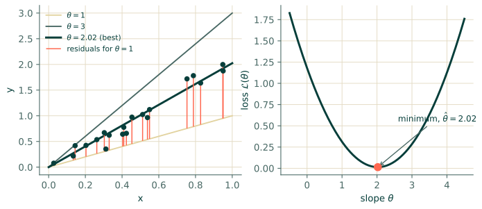
Take the simplest model with a single parameter, $f_\theta(x) = \theta x$ (a line through the origin), and data generated from $y = 2x$ plus noise. With one parameter the loss is a curve we can plot.

import numpy as np

rng = np.random.default_rng(1)
x = rng.uniform(0, 1, 20)
y = 2.0 * x + 0.1 * rng.normal(size=x.size)

def mse(theta):
    return np.mean((theta * x - y) ** 2)

for theta in [0.0, 1.0, 2.0, 3.0, 4.0]:
    print(f"theta = {theta:.1f}   loss = {mse(theta):.4f}")

theta = 0.0   loss = 1.1798
theta = 1.0   loss = 0.3122
theta = 2.0   loss = 0.0140
theta = 3.0   loss = 0.2851
theta = 4.0   loss = 1.1256

The loss is a parabola in $\theta$ (Figure 1.2, right), because it is a sum of squares of things that are linear in $\theta$. Its lowest point is where the slope of the curve is zero:

$$\frac{d\mathcal{L}}{d\theta} = \frac{2}{N}\sum_i (\theta x_i - y_i)\,x_i = 0 \quad\Longrightarrow\quad \hat\theta = \frac{\sum_i x_i y_i}{\sum_i x_i^2}.$$

theta_hat = np.sum(x * y) / np.sum(x ** 2)
print("closed form  theta_hat =", round(theta_hat, 4))
print("loss there            =", round(mse(theta_hat), 5))

# Nudge it either way: the loss can only go up.
print("loss at theta_hat -/+ 0.05:", round(mse(theta_hat - 0.05), 5), round(mse(theta_hat + 0.05), 5))

closed form  theta_hat = 2.0238
loss there            = 0.01379
loss at theta_hat -/+ 0.05: 0.0145 0.0145

Many parameters: least squares

A line with an intercept has two parameters, and the loss becomes a bowl in three dimensions. For any model that is linear in its parameters (lines, polynomials, and the last layer of a network) the bottom of the bowl has a closed form. Stack the inputs into a matrix $X$ whose rows are $(1, x_i, x_i^2, \dots)$; then $\mathcal{L} = \frac1N\lVert X\theta - y\rVert^2$ and setting the gradient to zero gives the normal equations

$$X^\top X\,\theta = X^\top y.$$

rng = np.random.default_rng(0)
x = np.sort(rng.uniform(0, 1, 12))
y = np.sin(2 * np.pi * x) + 0.15 * rng.normal(size=x.size)

X = np.vander(x, 4)                       # columns x^3, x^2, x, 1
theta, *_ = np.linalg.lstsq(X, y, rcond=None)

grad = 2 / len(x) * X.T @ (X @ theta - y)  # gradient of the MSE at the solution
print("theta =", np.round(theta, 2))
print("largest gradient component:", f"{np.abs(grad).max():.1e}")

theta = [ 21.59 -32.06  11.    -0.26]
largest gradient component: 9.7e-15

These are the same coefficients np.polyfit gave in Section 1.1: it was solving this problem all along. The gradient at the answer is zero to rounding error, which is the definition of "bottom of the bowl".

Neural networks are not linear in their parameters, so there is no closed form and we must search for the bottom step by step. That is Chapter 3. The loss, though, is the same object.

A loss does not need labels

Here is the idea that the rest of the book is built on. Nothing about the mean squared error requires $y_i$ to be a measurement. All it needs is a number $r_i$ that should be zero when the model is right. Measurements give one such number, "model minus data". A differential equation gives another.

Consider the equation $u'(x) = -u(x)$. If $u$ solves it then $r(x) = u'(x) + u(x)$ is zero for every $x$. So we can score any candidate function, with no data at all, by how far its residual is from zero:

xs = np.linspace(0, 1, 5)
candidates = {
    "exp(-x)": (np.exp(-xs), -np.exp(-xs)),     # (u, u')
    "1 - x":   (1 - xs,      -np.ones_like(xs)),
}
for name, (u, du) in candidates.items():
    r = du + u
    print(f"{name:8s} residual = {np.round(r, 3)}   mean r^2 = {np.mean(r**2):.4f}")

exp(-x)  residual = [0. 0. 0. 0. 0.]   mean r^2 = 0.0000
1 - x    residual = [ 0.   -0.25 -0.5  -0.75 -1.  ]   mean r^2 = 0.3750

The true solution scores exactly zero; the plausible-looking line $1 - x$ does not. That is a residual loss, and Chapter 6 develops it properly.

Exercises

1. Compute by hand the MSE of the model $f(x) = 2x$ on the three points $(1, 2.5)$, $(2, 3.5)$, $(3, 6.5)$.
2. Why can the normal equations fail for a degree-11 polynomial fitted to only 12 points and nearly equal $x$ values? (Hint: what does $X^\top X$ look like when two columns are almost parallel?)

Recap

• The loss is a single number, zero when the model is perfect; MSE is the mean of squared residuals.
• For models linear in their parameters, the minimum is found by solving the normal equations.
• A residual is any quantity that should be zero. A differential equation supplies one, with no labels needed.