Training a network end to end

We now have all the parts: a network (Chapter 2), a loss (Chapter 1), gradients by backpropagation, and an optimiser (this chapter). This section assembles them into the loop you will see, in some form, in every piece of PyTorch training code, including what the Lab generates.

The task

Learn $g(x) = \sin(2\pi x)$ on $[0, 1]$ from 25 evenly spaced values, with no noise. Afterwards, measure the error on 400 points the network never saw during training, as Section 1.3 taught us to.

The loop

import torch
import torch.nn as nn

class MLP(nn.Module):
    def __init__(self, sizes):
        super().__init__()
        self.layers = nn.ModuleList(nn.Linear(a, b) for a, b in zip(sizes[:-1], sizes[1:]))

    def forward(self, x):
        for layer in self.layers[:-1]:
            x = torch.tanh(layer(x))
        return self.layers[-1](x)

g = lambda x: torch.sin(2 * torch.pi * x)
x_train = torch.linspace(0, 1, 25).reshape(-1, 1)      # shape (N, 1): one row per point
y_train = g(x_train)
x_test = torch.linspace(0, 1, 400).reshape(-1, 1)
y_test = g(x_test)

def train(lr, decay=None, epochs=3000, seed=0):
    torch.manual_seed(seed)
    net = MLP([1, 20, 20, 1])
    opt = torch.optim.Adam(net.parameters(), lr=lr)
    sched = torch.optim.lr_scheduler.ExponentialLR(opt, gamma=decay) if decay else None
    history = []
    for epoch in range(epochs + 1):
        opt.zero_grad()                                   # 1. forget the last gradient
        loss = ((net(x_train) - y_train) ** 2).mean()     # 2. forward pass and loss
        loss.backward()                                   # 3. backpropagate
        opt.step()                                        # 4. move the weights
        if sched:
            sched.step()                                  # (optional) shrink the learning rate
        history.append(loss.item())
    with torch.no_grad():
        test_error = (net(x_test) - y_test).abs().max().item()
    return net, history, test_error

net, hist, err = train(lr=1e-2)
for epoch in [0, 10, 100, 500, 1000, 2000, 3000]:
    print(f"epoch {epoch:4d}   training loss {hist[epoch]:.2e}")
print(f"largest error on the 400 unseen points: {err:.4f}")

epoch    0   training loss 5.08e-01
epoch   10   training loss 2.52e-01
epoch  100   training loss 1.47e-01
epoch  500   training loss 4.98e-06
epoch 1000   training loss 5.72e-06
epoch 2000   training loss 8.95e-04
epoch 3000   training loss 6.58e-06
largest error on the 400 unseen points: 0.0076

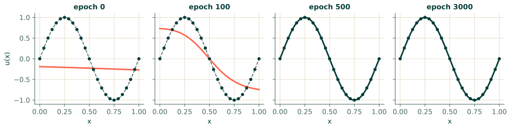
Four lines inside the loop carry all of the machinery of the chapter; compare them to the three-call pattern from Section 3.4. The loss falls from $0.5$ to the order of $10^{-6}$, and the network is within about a hundredth of the true curve even between the training points. Figure 3.7 shows the fit improving.

Habit 1: look at the whole loss curve, not just the end

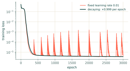
The printout above samples only seven epochs. A loss that is small at the end can hide a bumpy journey. Count how often, after the first 500 epochs, the loss jumped above $10^{-4}$:

spikes = sum(l > 1e-4 for l in hist[500:])
print("epochs after 500 with loss above 1e-4:", spikes, "of", len(hist[500:]))

epochs after 500 with loss above 1e-4: 192 of 2501

Plenty. With a fixed learning rate of $10^{-2}$, Adam keeps taking steps that are a little too big once it is close to the minimum, kicks the loss up, and recovers. The network is not broken, but the run is not converging cleanly either.

Habit 2: let the learning rate decay

A learning-rate schedule shrinks $\eta$ as training goes on: big steps to make fast progress at first, small steps to settle. The simplest is exponential decay, $\eta_k = \eta_0\,\gamma^k$. With $\gamma = 0.999$ the rate halves about every 700 epochs.

net2, hist2, err2 = train(lr=1e-2, decay=0.999)
print("fixed rate     : final loss", f"{hist[-1]:.1e}", "  spikes", sum(l > 1e-4 for l in hist[500:]),
      "  max test error", round(err, 4))
print("decaying rate  : final loss", f"{hist2[-1]:.1e}", "  spikes", sum(l > 1e-4 for l in hist2[500:]),
      "  max test error", round(err2, 4))

fixed rate     : final loss 6.6e-06   spikes 192   max test error 0.0076
decaying rate  : final loss 3.7e-06   spikes 0   max test error 0.004

No spikes, and a smaller final error. We changed nothing about the model or the data: only how the steps were taken. This is the pattern for the rest of the book. When training misbehaves, the first things to look at are usually the optimiser settings and the loss curve, before blaming the model.

From here to a PINN

Look at what this loop needed from the world: pairs $(x_i, y_i)$ and a rule for turning a mismatch into a number. The loop knows nothing about sine waves. Replace the line loss = ((net(x_train) - y_train) ** 2).mean() by a different function of the network, one that is small when the network satisfies a differential equation, and the very same loop, the same optimiser, the same backpropagation, trains a PINN. All that is missing is a way to compute derivatives of the network's output with respect to its inputs, because the equation is written in terms of them. That is Part 2.

Exercises

1. In the loop, what goes wrong if you delete opt.zero_grad()? Predict, then try it.
2. Change MLP([1, 20, 20, 1]) to MLP([1, 5, 1]). Do you expect the final error to rise or fall? Why?
3. Why is the error measured on x_test and not on x_train?

Recap

• A training loop is four steps repeated: zero the gradients, compute the loss, backpropagate, take an optimiser step.
• Look at the whole loss curve; a fixed learning rate may spike near the minimum, and a decaying schedule smooths it.
• The loop is indifferent to what the loss means. Changing the loss from "match the data" to "satisfy the equation" is what turns it into a PINN.