Scientific ML Studio

You now have the vocabulary: data, model, parameters, loss, generalisation. Before building the model itself, here is the map of where this book is going and why.

Three sources of information

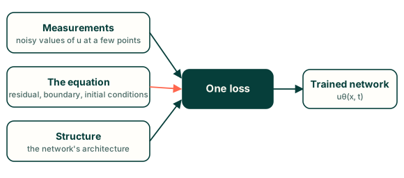
When you set out to find a physical field, say the temperature along a rod or the deflection of a beam, you can draw on three kinds of knowledge.

Measurements. Values of the field at some points, probably noisy.
The governing equation. A differential equation and its boundary and initial conditions, which say what kind of function the field must be.
Structure in the answer. Smoothness, symmetry, a known shape. This is what a model's architecture encodes.

Different methods lean on different mixtures.

	Measurements	Equation	Needs a mesh?	What you obtain
Classical solver (finite differences, finite elements)	no	yes	yes	The field at mesh nodes
Supervised neural network	yes, lots	no	no	A function fitted to the data
Physics-informed neural network	optional, few	yes	no	A function that is a network

The last column matters more than it looks. A classical solver returns numbers at nodes. A PINN returns a function $u_\theta(x, t)$ that you can evaluate at any point, differentiate exactly (Chapter 5), and carry over to a different question by changing a parameter.

Figure 1.5. A PINN uses all three sources at once. Each becomes a term in a single loss that the training loop minimises.

What a PINN does, in one paragraph

Pick a neural network $u_\theta(x, t)$ as the model. Write the differential equation as $\mathcal{N}[u] = 0$, where $\mathcal{N}$ collects its derivatives. Because $u_\theta$ is differentiable, the residual $r_\theta = \mathcal{N}[u_\theta]$ can be computed exactly at any point by automatic differentiation. Choose a set of points in the domain (collocation points), add penalties for violating the boundary and initial conditions, and for disagreeing with any measurements, and minimise the total. The loss is zero exactly when the network satisfies everything at once. This is the formulation of Raissi et al. (2019), and the next five chapters build it up piece by piece.

When is it the right tool?

Honesty first: for a clean, well-posed forward problem on a simple domain, a mature finite-element or finite-difference code is usually faster and more accurate than a PINN, and it comes with decades of error theory. PINNs earn their place elsewhere:

Inverse problems, where some coefficient or source in the equation is unknown and measurements are used to find it. The unknown becomes one more trainable parameter.
Sparse or irregular data that needs to be reconciled with a known law.
No mesh: awkward geometry, moving boundaries, or parametric studies where meshing for every variation is the bottleneck.
Differentiable solutions: derivatives of the answer with respect to inputs or parameters come for free.

PINNs have also been used for solid-mechanics problems. For instance, Fallah & Aghdam (2024) apply the idea to the bending and free vibration of a functionally graded porous beam on an elastic foundation; the reference list at the foot of this page links to the paper. We will not need their specific problem in this book, but it shows the kind of engineering setting where the governing equations are known and a mesh-free representation is attractive.

Training can fail

A PINN is trained by an optimisation that can stall, or converge to a function that nearly satisfies the equation in the wrong way. Much of Part 4 is about recognising and fixing that. If a loss curve goes down and the answer is still wrong, the method is not broken: the problem is usually in how the loss is balanced, the points are chosen, or the network is built.

The route through this book

Part	Chapters	You will be able to
1. AI and neural networks from zero	1–3	Read and write a small network and train it by gradient descent
2. Equations for ML people	4–5	Classify a PDE and differentiate a network with respect to its inputs
3. PINN fundamentals	6–8	Write a complete PINN, choose its points, handle time and unknowns
4. Making it work	9–12	Choose optimisers, balance the loss, pick architectures, diagnose failures
5. Worked problems	13	Reproduce full problems and compare to the Lab's generated code

Parts are released as they are finished, so later chapters will appear in the sidebar over time.

Exercises

For each situation, name the method from the table that fits best: (a) a rod's temperature, fully specified equation and boundary data, no measurements; (b) 50,000 labelled images; (c) an unknown thermal conductivity to be found from five thermometer readings.
In your own words, what does the residual of a differential equation measure?

Answers

(a) Classical solver, or a PINN if you want a differentiable function without a mesh. (b) A supervised network. (c) A PINN used as an inverse method: the conductivity is a trainable parameter, the equation supplies the structure, and the five readings supply the data.
How far a candidate function is from satisfying the equation at a point. It is zero where the function obeys the law and non-zero where it does not.

Recap

Measurements, equations and structure are three sources of information; a PINN uses all three through one loss.
A PINN returns a differentiable function, not numbers on a mesh, and is strongest for inverse problems and sparse data.
It is not automatically better than a classical solver, and training can fail. The later parts show how to cope.

Where PINNs fit

References

- Fallah, A., & Aghdam, M. M. (2024). Physics-informed neural network for bending and free vibration analysis of three-dimensional functionally graded porous beam resting on elastic foundation. Engineering with Computers, 40(1), 437–454. doi:10.1007/s00366-023-01799-7
- Raissi, M., Perdikaris, P., & Karniadakis, G. E. (2019). Physics-informed neural networks: A deep learning framework for solving forward and inverse problems involving nonlinear partial differential equations. Journal of Computational Physics, 378, 686–707. doi:10.1016/j.jcp.2018.10.045