Backpropagation
Gradient descent needs the gradient of the loss with respect to every weight. The chain rule, applied backwards through the network, delivers all of them for about the price of one extra forward pass.
For a polynomial we could write the gradient by hand. A network with thousands of weights has thousands of partial derivatives, and we need them at every step. Backpropagation is the algorithm that computes them all efficiently. It is nothing more than the chain rule, organised well. The idea of training layered networks this way was popularised by Rumelhart et al. (1986), and it has been the workhorse of the field since.
The chain rule in one line
If $y = f(g(x))$, then $\dfrac{dy}{dx} = f'(g(x))\cdot g'(x)$. A long chain multiplies the local slopes:
$$\frac{d\mathcal{L}}{d\theta} = \frac{d\mathcal{L}}{d\hat y}\cdot\frac{d\hat y}{dh}\cdot\frac{dh}{dz}\cdot\frac{dz}{d\theta}.$$
The strategy is to compute each local slope once, and reuse the running product. We will do it on the smallest network that shows everything.
A network small enough to differentiate by hand
One input, one hidden neuron with $\tanh$, one output, and a squared-error loss for a single example $(x, y)$:
$$z = w_1 x + b_1,\qquad h = \tanh z,\qquad \hat y = w_2 h + b_2,\qquad \mathcal{L} = \tfrac12(\hat y - y)^2.$$
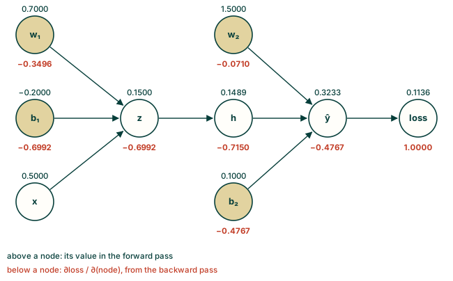
Forward pass. Compute the nodes in order and remember their values: they are needed again on the way back.
Backward pass. Start at the loss, where $\partial\mathcal{L}/\partial\mathcal{L} = 1$, and walk the graph in reverse. At each node, the gradient arriving from above is multiplied by that node's local slope, then passed down:
| node | local slope | gradient arriving at the node |
|---|---|---|
| $\hat y$ | $\partial\mathcal{L}/\partial\hat y = \hat y - y$ | $\bar{\hat y} = \hat y - y$ |
| $w_2,\ b_2$ | $\partial\hat y/\partial w_2 = h,\ \ \partial\hat y/\partial b_2 = 1$ | $\bar w_2 = \bar{\hat y}\,h,\ \ \bar b_2 = \bar{\hat y}$ |
| $h$ | $\partial\hat y/\partial h = w_2$ | $\bar h = \bar{\hat y}\,w_2$ |
| $z$ | $\partial h/\partial z = 1 - \tanh^2 z$ | $\bar z = \bar h\,(1 - h^2)$ |
| $w_1,\ b_1$ | $\partial z/\partial w_1 = x,\ \ \partial z/\partial b_1 = 1$ | $\bar w_1 = \bar z\,x,\ \ \bar b_1 = \bar z$ |
(The bar $\bar{\,\cdot\,}$ is shorthand for "the derivative of the loss with respect to this".) Notice how the tanh derivative $1 - h^2$ is computed from the value $h$ that the forward pass already stored. Here it is as code, checked two independent ways: against finite differences, and against PyTorch.
import numpy as np
import torch

x, y = 0.5, 0.8
w1, b1, w2, b2 = 0.7, -0.2, 1.5, 0.1

# forward
z = w1 * x + b1
h = np.tanh(z)
y_hat = w2 * h + b2
L = 0.5 * (y_hat - y) ** 2

# backward
d_yhat = y_hat - y
d_w2, d_b2 = d_yhat * h, d_yhat
d_h = d_yhat * w2
d_z = d_h * (1 - h ** 2)
d_w1, d_b1 = d_z * x, d_z

print(f"forward : z={z:.4f}  h={h:.4f}  y_hat={y_hat:.4f}  loss={L:.4f}")
backprop = np.array([d_w1, d_b1, d_w2, d_b2])
print("backprop:", backprop.round(4))

# check 1: finite differences
def loss_of(p):
    w1, b1, w2, b2 = p
    return 0.5 * (w2 * np.tanh(w1 * x + b1) + b2 - y) ** 2

p0 = np.array([w1, b1, w2, b2])
fd = np.array([(loss_of(p0 + e) - loss_of(p0 - e)) / 2e-6 for e in 1e-6 * np.eye(4)])
print("finite  :", fd.round(4))

# check 2: PyTorch's automatic differentiation
params = [torch.tensor(v, dtype=torch.float64, requires_grad=True) for v in p0]
t_w1, t_b1, t_w2, t_b2 = params
loss = 0.5 * (t_w2 * torch.tanh(t_w1 * x + t_b1) + t_b2 - y) ** 2
loss.backward()
print("autograd:", np.array([p.grad.item() for p in params]).round(4))
forward : z=0.1500  h=0.1489  y_hat=0.3233  loss=0.1136
backprop: [-0.3496 -0.6992 -0.071  -0.4767]
finite  : [-0.3496 -0.6992 -0.071  -0.4767]
autograd: [-0.3496 -0.6992 -0.071  -0.4767]
Three routes, one answer. The hand-written backward pass and PyTorch's loss.backward() are doing the same
arithmetic; the finite differences are a slow, independent referee. Making this kind of check a habit is
worthwhile: it is the quickest way to catch a bug in a loss you wrote yourself, and the loss of a PINN is
exactly such a thing.
Why backwards?
One might also compute derivatives by sweeping forward, tracking how each node changes with a given parameter. That costs one sweep per parameter. The backward sweep computes the derivative of one output (the loss) with respect to all parameters in a single sweep. With thousands of parameters and one scalar loss, the backward direction is the right one, and the cost is a small multiple of the forward pass whatever the number of parameters. The general technique is called reverse-mode automatic differentiation; Baydin et al. (2018) survey it and its forward-mode sibling. Backpropagation is its application to neural network training.
Forward mode has its own uses, for example when there are few inputs and many outputs. Chapter 5 puts the same backward machinery to a different job: instead of differentiating the loss with respect to the weights, we differentiate the network's output with respect to its inputs, which is the quantity a PDE residual needs.
For a whole layer
The same bookkeeping for a layer $\mathbf{z} = W\mathbf{a} + \mathbf{b}$, $\mathbf{h} = \sigma(\mathbf{z})$ gives, with $\bar{\mathbf{h}}$ the gradient arriving from above,
$$\bar{\mathbf{z}} = \bar{\mathbf{h}} \odot \sigma'(\mathbf{z}),\qquad \bar W = \bar{\mathbf{z}}\,\mathbf{a}^\top,\qquad \bar{\mathbf{b}} = \bar{\mathbf{z}},\qquad \bar{\mathbf{a}} = W^\top\bar{\mathbf{z}},$$
where $\odot$ is element-wise multiplication. The last line hands the gradient to the previous layer, and the recursion continues to the first. You will never write this yourself, but it shows the pattern: one matrix–vector product per layer in each direction.
The PyTorch pattern
In PyTorch, a training step is always the same three calls:
optimizer.zero_grad(): erase the old gradients (PyTorch accumulates into.grad, it does not overwrite).loss.backward(): run the backward pass, filling every parameter's.grad.optimizer.step(): update each parameter using its.grad, e.g. $\theta \leftarrow \theta - \eta\,\texttt{.grad}$.
Forgetting step 1 is the most common training bug: the gradients silently add up across iterations. The next two sections put this pattern to work.
Exercises
- In the table, what would $\bar w_1$ be if the activation were the identity ($h = z$)?
- With the numbers above, one gradient-descent step with $\eta = 0.5$ changes $w_2$ from $1.5$ to what? Does the loss go down?
- Why must the forward pass store $h$ and not just the final loss?
Answers
- The factor $1 - h^2$ becomes 1, so $\bar w_1 = \bar{\hat y}\, w_2\, x$.
- With $\bar w_2 \approx -0.071$: $w_2 \leftarrow 1.5 - 0.5(-0.071) \approx 1.536$. Increasing $w_2$ pushes $\hat y$ (currently below the target $0.8$) upwards, so the loss falls.
- The backward pass needs $h$ (for $\bar w_2$ and for $1 - h^2$). Without it the local slopes cannot be evaluated. Storing these intermediate values is why training uses more memory than inference.
Recap
- Backpropagation applies the chain rule backwards through the computational graph, multiplying local slopes.
- One backward sweep yields the gradient with respect to all parameters, which is why it scales to thousands.
- Check a hand-written gradient against finite differences, and in PyTorch remember
zero_grad→backward→step.
References
- Baydin, A. G., Pearlmutter, B. A., Radul, A. A., & Siskind, J. M. (2018). Automatic differentiation in machine learning: a survey. Journal of Machine Learning Research, 18(153), 1–43. https://jmlr.org/papers/v18/17-468.html
- Rumelhart, D. E., Hinton, G. E., & Williams, R. J. (1986). Learning representations by back-propagating errors. Nature, 323(6088), 533–536. doi:10.1038/323533a0