Poisson on a square
The same idea on the unit square: two derivatives, four edges, and a lesson that does not show up in one dimension. How you weight the boundary against the equation changes the answer. A finite-element solution gives an independent check.
In one dimension the boundary was two points, and equal weights worked. On a square the boundary is four curves, each sampled with many points, and the equation term and the boundary terms are no longer of comparable size. This page shows what that does, with a pair of runs that differ in nothing but one number.
It is also where we set the PINN beside something independent: the exact solution, and a finite-element solution computed on a mesh.
1. The problem
Find $u(x,y)$ on the unit square $\Omega = (0,1)^2$ such that
$$ -\nabla^2 u = 2\pi^2\sin(\pi x)\sin(\pi y), \qquad u = 0 \text{ on all four edges.} $$
Here $\nabla^2 u = u_{xx} + u_{yy}$. Physically, $u$ is the steady temperature of a thin square plate with its edges held at zero and a heat source warming the middle.
The exact answer is $u = \sin(\pi x)\sin(\pi y)$. Each second derivative of it brings down a factor $-\pi^2$, so $-\nabla^2 u = 2\pi^2\sin(\pi x)\sin(\pi y)$, and it vanishes on every edge because $\sin 0 = \sin\pi = 0$.
The sign in the Lab
The Lab's Poisson block solves $\nabla^2 u = f$. For $-\nabla^2 u = 2\pi^2\sin(\pi x)\sin(\pi y)$ you enter $f = -2\pi^2\sin(\pi x)\sin(\pi y)$, which in the Lab's notation is -2*pi**2*sin(pi*x)*sin(pi*y). This is exactly the source of the Lab's Poisson on a square starter.
2. What changes from one dimension
The network $u_\theta(x, y)$ now has two inputs, and the residual needs both second derivatives, each by automatic differentiation:
$$ r_\theta(x,y) = \frac{\partial^2 u_\theta}{\partial x^2} + \frac{\partial^2 u_\theta}{\partial y^2} - f(x,y). $$
The loss has one PDE term and one term per edge:
$$ \mathcal{L}(\theta) = w_{\text{pde}}\,\overline{r_\theta^2} \;+\; \sum_{k=1}^{4} w_{k}\,\overline{u_\theta^2}\Big|_{\text{edge }k}, $$
where the overlines are means over that term's points. Three things are new: two derivatives, a boundary made of four sampled edges, and four weights $w_k$ that now matter.
3. In the Lab
This is the Lab's Poisson on a square starter with one change, the boundary weights.
| Block | Setting |
|---|---|
| Domain | Rectangle, $x, y \in [0, 1]$, no time. 2000 interior points, 80 per edge |
| PDE | Elliptic → Poisson, source -2*pi**2*sin(pi*x)*sin(pi*y) |
| BC 1–4 | Dirichlet, u = 0.0, on the left, right, bottom and top edges |
| Network | 40, 40, 40, 40, tanh, Xavier (5,081 parameters) |
| Loss | Mean square, PDE weight 1, BC weights [100, 100, 100, 100] |
| Optimiser | Adam, learning rate 0.001, 5000 epochs |
Download the finished notebook, poisson-2d.omega-notebook.json, and open it with Open a notebook file… on the Lab page. The scripts it generates are poisson_2d_w100.py, and poisson_2d_w1.py for the same notebook with all weights at 1. They differ in one line, the TERM_SCALES dictionary, where the weights end up:
# not run
TERM_SCALES = {'pde1': 1.0, 'bc1': 100.0, 'bc2': 100.0, 'bc3': 100.0, 'bc4': 100.0}
4. The result
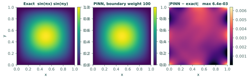
We ran the Lab's script (boundary weight 100) three times, changing only the seed that sets the starting weights. The relative $L^2$ error against the exact answer, on a $101\times101$ grid that is not the set of training points, was $5.7\times10^{-3}$, $7.6\times10^{-3}$ and $3.0\times10^{-3}$. The largest pointwise errors were $6.4\times10^{-3}$, $7.3\times10^{-3}$ and $3.5\times10^{-3}$. Each run took about 70 seconds on the two-core cloud machine we used.
The network is never wrong by much: a hill of height 1, reproduced to within less than a percent. Figure 13.3 shows one run. The error map, on the right, is the useful panel. It says where the error lives, which a single number cannot.
5. Why the boundary weight matters
Run the same notebook with the boundary weights at 1 instead of 100, and nothing else changed. Three seeds each:
| Boundary weight | Seed | Relative $L^2$ error | Largest pointwise error | Where the largest error is |
|---|---|---|---|---|
| 1 | 1 | $6.0\times10^{-3}$ | $1.9\times10^{-2}$ | a corner |
| 1 | 2 | $1.1\times10^{-2}$ | $2.4\times10^{-2}$ | a corner |
| 1 | 3 | $8.0\times10^{-3}$ | $2.1\times10^{-2}$ | a corner |
| 100 | 1 | $5.7\times10^{-3}$ | $6.4\times10^{-3}$ | a corner |
| 100 | 2 | $7.6\times10^{-3}$ | $7.3\times10^{-3}$ | an edge |
| 100 | 3 | $3.0\times10^{-3}$ | $3.5\times10^{-3}$ | an edge |
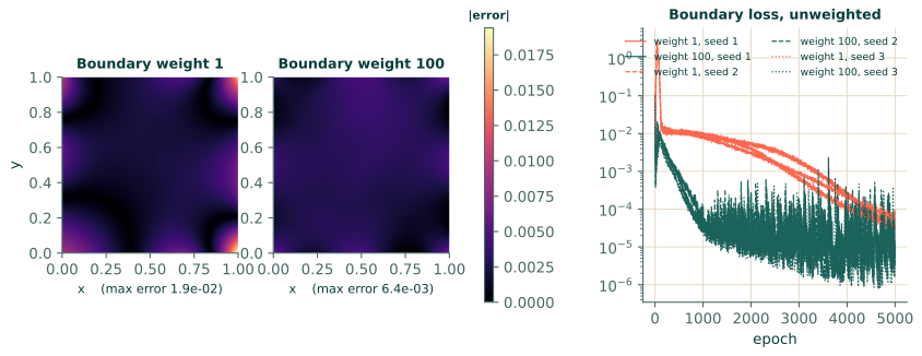
Two things stand out, and they should be kept separate. The worst error drops by a factor of 3 to 6 with the larger weight. The overall error improves less, and unevenly: hardly at all for seed 1, and about 2.7 times lower for seed 3. With only three seeds each, do not read more into the overall figure than that. What is the same in all six runs is that the worst place is on the boundary, and with weight 1 it is always a corner.
The right-hand panel of Figure 13.4 shows why. At the first epoch the equation term is about 100 and the boundary term about 0.1, a thousand times smaller, so the optimiser spends its early effort on the equation. With weight 1 the boundary loss is still about $10^{-2}$ at epoch 1000. With weight 100 it is about $5\times10^{-5}$ by then, at the price of an equation term that is several times larger at that moment. The edges are enforced sooner, and the equation catches up later.
The cause is that the equation loss and the boundary losses are different quantities with different sizes, and nothing in the method says they should be equal. See why the weights matter. If the loss falls but the answer is worst along the edges, raise the weight on those edges by a factor of ten and run again.
6. A check that is not the exact answer
An exact solution is a luxury. For a PINN to be trusted on a problem without one, it has to agree with an independent method. For this problem, the finite-element method (FEM) with bilinear (Q1) elements on a structured mesh is that method, and its error is well understood: it falls like $h^2$, where $h$ is the element size.
| Mesh | Element size $h$ | Relative $L^2$ error | Observed order |
|---|---|---|---|
| $4\times4$ | 0.250 | $6.1\times10^{-2}$ | |
| $8\times8$ | 0.125 | $1.5\times10^{-2}$ | 2.0 |
| $16\times16$ | 0.0625 | $3.8\times10^{-3}$ | 2.0 |
| $32\times32$ | 0.0312 | $9.5\times10^{-4}$ | 2.0 |
| $64\times64$ | 0.0156 | $2.4\times10^{-4}$ | 2.0 |
Errors are measured on the same $101\times101$ grid used for the PINN. (The source term is a product of sines, so its integrals against the element basis can be done exactly, which flatters the FEM a little. A general source would need quadrature.) Every one of these solves took well under a tenth of a second on the same machine.
Against that, the PINN's three errors with boundary weight 100, $3.0\times10^{-3}$ to $7.6\times10^{-3}$, sit between the $8\times8$ and $32\times32$ meshes, mostly between $8\times8$ and $16\times16$, and took about 70 seconds each.
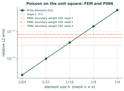
Read this comparison carefully. It rests on a few runs, and the PINN's error moves from run to run. The costs are different in kind: the FEM time is the assembly and solve of a sparse linear system, the PINN time is five thousand epochs of optimisation. And the strengths are different. The FEM needs a mesh; a PINN is mesh-free, gives a continuous function, and can fold in measured data. A fair comparison of your own should use the same test grid and error measure for both, several seeds for the PINN, and honest timings.
The FEM column was computed by the fem_q1 function in the site's tools/figures_examples.py, about thirty lines of NumPy and SciPy.
7. Exercises
- A different mode. Set $f = -5\pi^2\sin(2\pi x)\sin(\pi y)$. What is the exact solution? (Only the PDE block changes.)
- Fewer points. Cut the interior points to 400. How does the error between the training points change?
- The weights. Try BC weights of 10 and 1000. Is there a point where raising the weight stops helping?
- Different weights per edge. The Loss block accepts a different number for each edge. Give the top edge weight 100 and the others 1. Where is the error now?
Answer to 1
$u = \sin(2\pi x)\sin(\pi y)$. Each $x$-derivative twice brings down $-(2\pi)^2$ and each $y$-derivative $-\pi^2$, so $\nabla^2 u = -(4\pi^2 + \pi^2)u = -5\pi^2 u$, which is $f$, and $u = 0$ on all four edges.
The others are to be run; judge them with several seeds and a separate grid.
8. Recap
- The 2D problem is the 1D idea with two inputs, four sampled edges and second derivatives in both directions.
- The Lab sign for Poisson is $\nabla^2 u = f$; for $-\nabla^2 u = g$ enter $f = -g$.
- Weight the boundary. Giving the four edges a weight of 100 brought the worst error down by a factor of 3 to 6 in our runs, and the corners stopped being the worst place. The overall error improved by much less. Choose the weight by looking at the error map and the boundary loss, not by habit.
- Judge a result by where the error is, not only how large it is, and compare against an independent reference.