Laplace's equation on a disc: a curved boundary
Leave the square behind. Solve a source-free equation on a circular domain, with boundary data given as a formula in x and y, and see how the maximum principle lets you check an answer without any reference solution.
Every domain so far was a line, a rectangle, or a square: shapes with straight edges and corners. Real problems are rarely so tidy. This guide moves to a disc, where the boundary is a single smooth curve, and it uses the simplest equation in all of physics, Laplace's equation, which has no source term at all.
It is a short, clean guide, and a good one to try right after the Poisson problems, because almost nothing else changes. What is new is the geometry, the way points are sampled in a curved region, and a useful property of the solution that lets you check your answer without ever computing it.
Before you start. Finish the two Poisson guides first, in particular Poisson on a square. Open the Studio and choose an empty canvas.
1. The problem
Find $u(x,y)$ inside the unit disc, $x^2+y^2<1$, such that
$$ \nabla^2 u = \frac{\partial^2 u}{\partial x^2} + \frac{\partial^2 u}{\partial y^2} = 0 \quad \text{inside the disc,} $$
and on the circle $x^2+y^2=1$ the value is prescribed by a formula,
$$ u = e^{x}\cos(y) \quad \text{on the circle.} $$
Physically, $u$ could be the steady temperature of a round metal plate whose rim is heated unevenly: hot on the right, cooler on the left. With no heat source inside, the temperature in the middle is entirely determined by what is happening on the rim. This is exactly Poisson's equation with $f = 0$, called Laplace's equation.
The exact answer
Try $u(x,y) = e^{x}\cos(y)$ everywhere in the disc. Then
$$ \frac{\partial^2 u}{\partial x^2} = e^{x}\cos y, \qquad \frac{\partial^2 u}{\partial y^2} = -e^{x}\cos y, $$
which add to zero. And on the circle it equals the prescribed data by construction. So
$$ u_{\text{exact}}(x,y) = e^{x}\cos(y). $$
Functions that satisfy Laplace's equation are called harmonic. This one was found with the same trick as in the manufactured-solutions guide: pick a harmonic function, then use its values on the boundary as the data.
A property you can use. A harmonic function has no hills or valleys in the interior. Its largest and smallest values are always found on the boundary (this is the maximum principle). Here the largest value is $e^{1}\approx 2.718$, at the point $(1,0)$ on the rim, and the smallest is $e^{-1}\approx 0.368$, at $(-1,0)$. If a trained network ever shows a bump in the middle of the disc that is higher than anything on the rim, it is wrong, and you know it without needing the exact answer.
2. How a PINN sees the problem
Two inputs, one output, and a residual that now has no source term:
$$ r_\theta(x,y) = \frac{\partial^2 u_\theta}{\partial x^2} + \frac{\partial^2 u_\theta}{\partial y^2}, $$
$$ \mathcal{L}(\theta) = \overline{r_\theta^{\,2}} \;+\; w_{\text{bc}}\;\overline{\bigl(u_\theta - e^{x}\cos y\bigr)^2_{\text{on the circle}}} . $$
Two details matter for the circle.
Sampling inside a disc. The collocation points must fall inside the disc, and they should be spread evenly by area. Sampling a radius and an angle uniformly looks reasonable but crowds points near the centre, because small circles have little area. The right recipe is to draw the radius as $r=\sqrt{\text{uniform}(0,1)}$ and the angle uniformly. The Studio does this for you when you choose a circular domain, but you should know it is happening, and check it if you ever write a script by hand.
The boundary is one closed curve. A square had four edges and needed four boundary conditions. A circle has one boundary, so there is one condition, with the data written as a formula in $x$ and $y$ evaluated at the points on the rim.
3. The plan: one block per decision
| # | Block | The question it answers | Our choice |
|---|---|---|---|
| 1 | DOM Domain | Where does the problem live? | Two space dimensions, circle of radius 1 centred at the origin, no time |
| 2 | PDE Equation | Which equation must hold inside? | Laplace, $\nabla^2 u = 0$ (Poisson with $f=0$) |
| 3 | BC Boundary | What is fixed on the rim? | One Dirichlet condition: $u = e^{x}\cos y$ |
| 4 | NET Network | What function family do we search in? | 2 inputs, 3 hidden layers of 32 neurons, $\tanh$, 1 output |
| 5 | LOSS Loss | How do we score the errors? | Mean squared error, weight 1 on the PDE and 100 on the boundary |
| 6 | OPT Optimiser | How do the weights change? | Adam, learning rate $10^{-3}$ |
| 7 | RUN Train | How long and with how many points? | 5000 epochs, about 1000 interior points, 200 on the circle |
A note on labels. The Studio's wording can differ slightly between versions. The quantity to set is what matters; if a field name does not match exactly, pick the nearest one. If a value is not offered, keep the Studio's default.
4. Step by step in the Studio
Step 1: Domain (DOM)
Add a Domain block. Choose a two-dimensional domain with the Circle geometry, radius 1, centred at (0, 0). Leave time off.
Check: the block shows a circle, not a rectangle. If it still lists $x$ and $y$ ranges as an interval each, you have a square domain, and the whole problem would be set on the wrong shape.
Step 2: Equation (PDE)
Add an Equation block, connect the Domain to it, and choose the Laplace equation. If your version of the Studio lists only Poisson, choose Poisson and set the source term to 0.
Check: the summary reads $\nabla^2 u = 0$, with no source term, or $f = 0$.
Step 3: Boundary condition (BC)
Add a Boundary block and connect the Domain to it. A circle has a single boundary, so add one Dirichlet condition:
| Where | Type | Value |
|---|---|---|
| The circle | Fixed value (Dirichlet) | exp(x)*cos(y) |
The value is an expression in the coordinates of the point on the rim. The Studio substitutes the $x$ and $y$ of each rim point into it.
Check: the Studio counts one boundary condition. A closed curve is one boundary, so a count of four would mean the domain is still a square.
Step 4: Network (NET)
Add a Network block, connect the Domain to it, and use 2 inputs, 3 hidden layers of 32 neurons, tanh, and 1 output.
Step 5: Loss (LOSS)
Add a Loss block, connect the Equation, Boundary and Network, use mean squared error, and set the weights to PDE = 1 and boundary = 100. With a single condition this is one number: if the Studio wants a list, enter [100]. Section 5 shows what a weight of 1 does instead.
Step 6: Optimiser and Train
Add an Optimiser block (Adam, learning rate 0.001) and a Train block (5000 epochs, about 1000 interior points and 200 points on the circle). Connect the Loss and Optimiser to Train.
Check: no warnings. A clean check means consistent, not accurate.
Step 7: Generate and run
Generate the Python code, download the script and run it on your own computer. The Studio builds and checks the configuration; training happens in your script. A run this size takes a couple of minutes on a laptop CPU.
Step 8: Judge the result
Compare with $e^{x}\cos y$ on a fine grid of points inside the disc that were not used for training. Here that is a $201\times201$ grid, keeping only the points with $x^2+y^2\le1$.
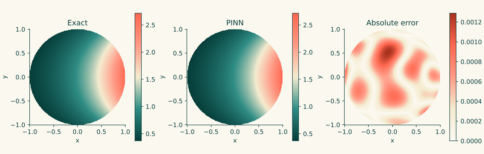
Two things to notice.
The solution is smooth and boring, and that is good. It is a gentle ramp from cool on the left to warm on the right. There are no layers or spikes. Laplace's equation produces the smoothest possible interior: every value is a kind of average of its neighbours.
The error is spread out. In earlier guides it concentrated on the edges, because the boundary was under-weighted. With a weight of 100 on the rim, the edge is matched very well and the leftover error is a scattering of soft patches over the whole disc. In the reference run the largest error in each ring of the disc was about the same: $8\times10^{-4}$ in the centre, about $1.2\times10^{-3}$ to $1.3\times10^{-3}$ at middle radii, and $1.0\times10^{-3}$ near the rim.
The maximum principle gives a second check that needs no exact answer. The PINN's smallest and largest values on the grid were 0.3669 and 2.7177, against the exact $0.3679$ and $2.7183$. The extremes sit on the rim and not inside, as they should.
The summary measure is the relative $L^2$ error over the disc,
$$ \varepsilon = \frac{\lVert u_\theta - u_{\text{exact}} \rVert_2}{\lVert u_{\text{exact}} \rVert_2}. $$
What to expect
These figures come from a hand-written reference implementation with exactly the settings above (random seed 0). The Studio's script may initialise and sample slightly differently, so your numbers will differ, but you should land in the same neighbourhood.
| Epoch | Total loss | Relative $L^2$ error |
|---|---|---|
| 0 | $2 \times 10^{2}$ | $1.1$ |
| 1000 | $9 \times 10^{-2}$ | $1.3 \times 10^{-2}$ |
| 3000 | $3 \times 10^{-3}$ | $1.1 \times 10^{-3}$ |
| 5000 | $7 \times 10^{-4}$ | $4.4 \times 10^{-4}$ |
The largest pointwise error at the end was about $1.3 \times 10^{-3}$, on a solution that ranges from 0.37 to 2.72.
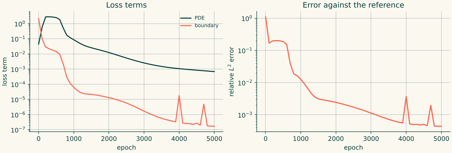
Keep the best result. Around epoch 4000 the error briefly rose to about $4\times10^{-3}$, from about $10^{-3}$ a thousand epochs earlier, before settling again. It is ordinary Adam behaviour on a PINN. A run that stops on a spike is a bad sample of a good method.
5. The boundary weight moves the error, it does not always shrink it
The same problem was run again with the boundary weight dropped from 100 to 1 and everything else unchanged.
| Boundary weight | Relative $L^2$ error after 5000 epochs | Largest error, rings of radius 0 to 0.2 | Largest error, ring of radius 0.8 to 1.0 |
|---|---|---|---|
| 1 | $3.7 \times 10^{-4}$ | $9 \times 10^{-5}$ | $2.2 \times 10^{-3}$ |
| 100 | $4.4 \times 10^{-4}$ | $8 \times 10^{-4}$ | $1.0 \times 10^{-3}$ |
This is a result worth stopping on, because it is not what the square-domain guide led you to expect. Both weights reached a similar overall error (these are single runs with one random seed, so $3.7\times10^{-4}$ against $4.4\times10^{-4}$ is a tie). What changed is where the error sits. With weight 1 the middle of the disc is very accurate, about $10^{-4}$, and the error piles up at the rim, where it is more than twenty times larger. With weight 100 the rim is matched much more tightly, and the error is spread evenly over the whole disc.
Two reasons this problem is so forgiving. First, the solution is gentle and the rim data is smooth, so the network can meet it without a fight. Second, Laplace's equation has no source term, so the PDE loss on its own pushes the network towards a smooth, almost-harmonic function, and the rim data then selects the right one. A bigger weight did not buy a better overall answer, but it did decide which part of the disc you can trust most. Pick the weight by looking at where you need the accuracy: if you care most about the rim values, raise the weight; if you care about the interior, a modest weight may serve better.
A habit to keep. Whenever you change a weight, look at the error map, not only the single summary number. Two runs with the same $L^2$ error can be wrong in very different places.
6. If something goes wrong
| What you see | Likely cause | What to try |
|---|---|---|
| The domain looks like a square, or the Studio asks for four boundary conditions | Domain is not set to the circle | Choose the Circle geometry in Step 1 |
| The extremes are in the middle of the disc | The answer is wrong (the maximum principle is violated) | Check the boundary expression and its weight |
| Error largest right at the rim | Boundary weight too low or too few rim points (the weight-1 run in Section 5 did this) | Raise the weight to 100, or use 400 rim points |
| A solution that is a mirror image | A sign or an $x$ and $y$ mix-up in the data | Re-enter exp(x)*cos(y) and check the symbols |
Loss is nan |
Learning rate too high, or a typo such as ^ for ** |
Lower to $10^{-4}$ and recheck the expression |
7. Try it yourself
- A different harmonic function. Use the data $u = x^2 - y^2$ on the circle. It is harmonic everywhere, so the exact solution is $x^2-y^2$ throughout the disc. Only the Boundary block changes.
- A circle with another size and centre. Use radius 2 and centre $(1,0)$, with the data $e^{x}\cos y$ still evaluated on the new rim. Is $e^{x}\cos y$ still the exact answer? Check that it still satisfies the equation.
- A rim that is not smooth. Try the data $u=|y|$ on the circle. It has two corners, at $(\pm1,0)$. Where does the PINN's error move to?
- A source term. Switch to Poisson with $f = 4$ and the rim data $u = 1$. The exact solution is $u = x^2+y^2$, whose Laplacian is 4 and which equals 1 on the rim. The solution is a bowl rising from 0 at the centre to 1 at the edge. Only the Equation and Boundary blocks change.
- Spot the unfair sampling. If you write a script by hand, sample the radius uniformly and the angle uniformly (no square root) and compare the error near the centre with the correct version.
8. Recap
- A disc is a Circle geometry in the Domain. It has one boundary, so it needs one boundary condition, with the data written as a formula in $x$ and $y$.
- Laplace's equation is Poisson's equation with no source: $\nabla^2 u = 0$. The interior is completely determined by the boundary.
- The solution of Laplace's equation has no interior maximum or minimum. Use this as a check that needs no exact answer.
- Sampling inside a circle must be uniform in area, which means taking the square root of the random radius.
- The boundary weight changes where the error sits as much as how big it is: weight 1 left the interior very accurate and the rim worse, weight 100 spread the error evenly. Look at the error map, not only the summary number.
Reference script for the numbers quoted above: laplace_disc_reference.py. It is written by hand for checking this guide and is not the Studio's generated output.