A standing wave: second derivatives in time

The heat equation relaxes: whatever you start with fades away. The wave equation is different. It never forgets. A plucked string vibrates, swings through its rest position, reaches the opposite extreme, and comes back, over and over. That makes it a harder test for a PINN, and a very informative one.

This guide solves the simplest wave problem there is, a standing wave on a string held at both ends, and it focuses on the three things that are new: a second derivative in time, an initial velocity condition, and a training curve with an awkward shape you should learn to recognise.

Before you start. Finish Heat in a bar first. This guide uses the same time-dependent set-up and goes faster. Open the Studio and choose an empty canvas.

1. The problem

A string of unit length is fixed at both ends. Let $u(x,t)$ be its sideways displacement. It obeys

$$ \frac{\partial^2 u}{\partial t^2} = c^2\,\frac{\partial^2 u}{\partial x^2}, \qquad 0

where $c$ is the wave speed. We take $c = 1$. The string starts from a smooth bump and is released from rest:

$$ u(x,0) = \sin(\pi x), \qquad \frac{\partial u}{\partial t}(x,0) = 0 , $$

and both ends stay fixed:

$$ u(0,t) = 0, \qquad u(1,t) = 0 . $$

Two initial conditions are needed, not one. The equation is second order in time, so, just as with a ball thrown in the air, you must say both where it is and how fast it is moving before the future is determined. Heat is first order in time and needed only the starting shape.

The exact answer

Try $u(x,t) = \cos(c\pi t)\,\sin(\pi x)$. The shape stays the same and only its height swings up and down:

$$ u_{tt} = -c^2\pi^2\cos(c\pi t)\sin(\pi x), \qquad u_{xx} = -\pi^2\cos(c\pi t)\sin(\pi x), $$

so $u_{tt} = c^2 u_{xx}$ holds. At $t=0$ it gives $\sin(\pi x)$, the velocity $u_t = -c\pi\sin(c\pi t)\sin(\pi x)$ is zero at $t=0$, and the sine vanishes at both ends. So

$$ u_{\text{exact}}(x,t) = \cos(\pi t)\,\sin(\pi x) \qquad (c=1). $$

With $c=1$ the string is at its top at $t=0$, flips to the bottom at $t=1$, and returns to the top at $t=2$. We train over $0\le t\le2$ so that the network has to follow one full oscillation.

2. How a PINN sees the problem

The network is again $u_\theta(x,t)$, with two inputs. The new parts of the loss are the second time derivative and the velocity condition.

The equation error.

$$ r_\theta(x,t) = \frac{\partial^2 u_\theta}{\partial t^2} - c^2\,\frac{\partial^2 u_\theta}{\partial x^2}, $$

two second derivatives, both by automatic differentiation.

The initial displacement and the initial velocity. At $t = 0$:

$$ u_\theta(x,0) = \sin(\pi x), \qquad \frac{\partial u_\theta}{\partial t}(x,0) = 0 . $$

The second one needs a first derivative of the network with respect to time, evaluated on the line $t=0$.

The boundary error. $u_\theta(0,t) = u_\theta(1,t) = 0$.

$$ \mathcal{L}(\theta) = \overline{r_\theta^{\,2}} + w_{\text{ic}}\Bigl[\overline{(u_\theta - \sin\pi x)^2}_{t=0} + \overline{(\partial_t u_\theta)^2}_{t=0}\Bigr] + w_{\text{bc}}\,\overline{u_\theta^{\,2}}_{\text{ends}} . $$

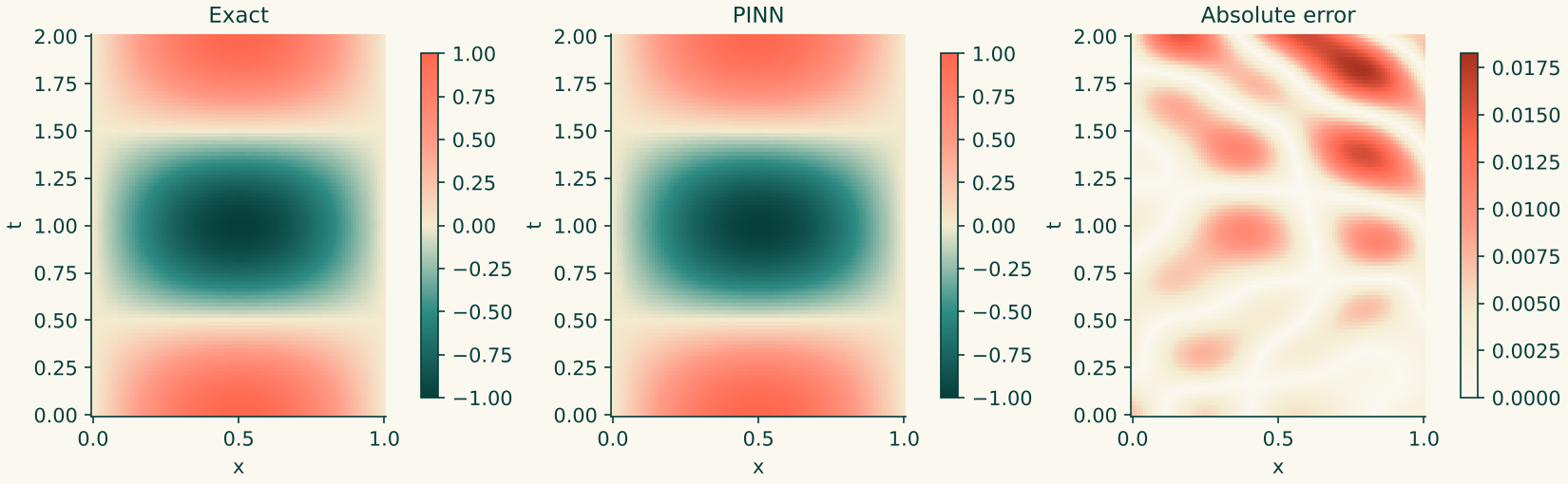
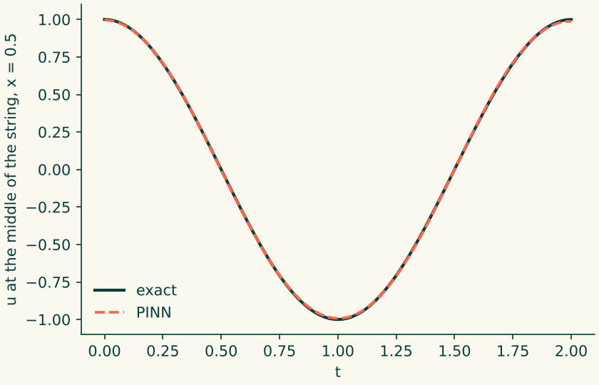
Why $\tanh$ matters even more. The residual contains $u_{tt}$ and $u_{xx}$, so, as in the Poisson guides, the network must have a meaningful second derivative. A smooth activation such as $\tanh$ is required. Do not use ReLU for any second-order equation.

3. The plan: one block per decision

A note on labels. The Studio's wording can differ slightly between versions. The quantity to set is what matters; if a field name does not match exactly, pick the nearest one. If a value is not offered, keep the Studio's default.

4. Step by step in the Studio

Step 1: Domain (DOM)

Add a Domain block: one-dimensional, $x$ from 0 to 1, time on, $t$ from 0 to 2.

Check: one space coordinate and a time axis that ends at 2.

Step 2: Equation (PDE)

Add an Equation block, connect the Domain to it, and choose the Wave equation. Set the speed $c$ to 1.

Check: the summary reads $u_{tt} = c^2 u_{xx}$.

Step 3: Boundary and initial conditions (BC)

Add a Boundary block, connect the Domain, and enter four conditions:

Check: the Studio counts four conditions. The wave equation needs the initial condition and the initial velocity. If you enter only the initial condition the Studio warns you, and the problem would be genuinely ambiguous: a string released from rest and one that was thrown both start from the same shape.

Step 4: Network (NET)

Add a Network block, connect the Domain, and use 2 inputs, 3 hidden layers of 32 neurons, tanh, and 1 output.

Step 5: Loss (LOSS)

Add a Loss block, connect the Equation, Boundary and Network, use mean squared error, set the PDE weight to 1 and the weights on the four conditions to 10. If the Studio asks for them as a list in the order above, enter [10, 10, 10, 10].

Step 6: Optimiser and Train

Add an Optimiser block (Adam, learning rate 0.001) and a Train block (6000 epochs, about 3000 interior points). Connect the Loss and Optimiser to Train.

Check: no warnings. A clean check means consistent, not accurate.

Step 7: Generate and run

Generate the Python code, download the script and run it on your own computer. The Studio builds and checks the configuration; training happens in your script. This is the slowest guide so far, because the residual involves two second derivatives: allow a few minutes on a laptop CPU.

Step 8: Judge the result

Compare with the exact solution on a $101\times101$ grid in $(x,t)$ that was not used for training.

The left two panels are a full oscillation: a bump, a trough, and a bump again. The error panel is the lesson. The error is small at the start and grows as time goes on. Here is the largest pointwise error at five times:

The errors are small in absolute terms, but they are about 2.4 times larger at the end than at the start. That is typical for evolution problems: the initial condition is imposed directly, while later times are reached only through the equation, so mistakes in one place feed into the next. A PINN has no time-stepping to accumulate error, yet the same drift shows up.

The middle of the string is a good single place to look. It should read $+1$ at $t=0$, $-1$ at $t=1$, and $+1$ again at $t=2$.

The reference run gave $0.996$, $-0.993$ and $0.987$. The peak slowly shrinks, a hint of numerical damping: the network has found a wave that is slightly too lazy.

The summary measure is the relative $L^2$ error over the whole $(x,t)$ grid,

$$ \varepsilon = \frac{\lVert u_\theta - u_{\text{exact}} \rVert_2}{\lVert u_{\text{exact}} \rVert_2}. $$

What to expect

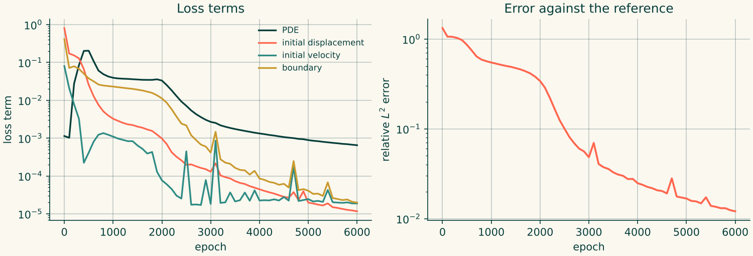
These figures come from a hand-written reference implementation with exactly the settings above (random seed 0). The Studio's script may initialise and sample slightly differently, so your numbers will differ, but you should land in the same neighbourhood.

The relative error ends near 1%. That is one decimal place worse than the heat equation, and it is the honest price of an oscillating solution.

5. The plateau: why the first 2000 epochs look stuck

Look at the training curves.

Three things stand out.

1. The PDE term starts tiny, then rises. At epoch 0 the network outputs almost zero everywhere, and a function that is zero everywhere satisfies $u_{tt} = c^2 u_{xx}$ trivially. The equation looks happy. As soon as the network starts bending to meet the initial shape, the equation term rises, to about 0.2 around epoch 400.
2. Then comes a plateau. For roughly 1500 epochs the loss and the error both hover on a shelf (error about 0.5). The network has the right initial bump but has not yet learned how it should move.
3. Then a sudden drop around epoch 2000, after which the error falls by an order of magnitude in about a thousand epochs.

Do not stop on the plateau. A flat curve in the loss does not mean the method has failed. It means the network is still looking for the way the solution moves. If you stopped at epoch 1500 you would have a total loss of a few tenths and an answer that is about 45% wrong. Always judge by the comparison with a reference, not by the loss alone. This is the clearest example in the whole series of a loss number that does not tell you the answer is right.

Run longer if the plateau has not broken. Longer time ranges are generally harder for PINNs on wave problems (this guide did not test one), and that is one reason practitioners often train over short time windows and chain them together.

6. If something goes wrong

7. Try it yourself

1. A faster wave. Set $c = 2$. The exact solution is $\cos(2\pi t)\sin(\pi x)$, which completes a full oscillation in $t=1$. Only the Equation block and the exact answer change. Does the PINN need more epochs?
2. A higher mode. Use the initial shape $\sin(2\pi x)$. The exact solution is $\cos(2\pi c t)\sin(2\pi x)$. Higher modes oscillate faster, so they are harder.
3. A string that is thrown. Start flat, $u(x,0)=0$, with initial velocity $u_t(x,0)=\pi\sin(\pi x)$. The exact solution is $\sin(\pi t)\sin(\pi x)$. This is the same equation with the two initial conditions swapped, and a good test of the velocity term.
4. A shorter window. Train on $t\in[0,0.5]$ only. How much smaller is the error?
5. Watch the plateau. Change the seed or the learning rate and see how long the plateau lasts.

8. Recap

• A wave equation is second order in time, so it needs two initial conditions: the shape and the velocity.
• A PINN reads the initial velocity from the network's time derivative at $t=0$.
• The PDE loss can start deceptively small, because "nothing happening" satisfies the equation. A low loss is not proof of a good answer.
• Expect a plateau early in training, and an error that grows with time: here it was about 1% overall, and about 2.4 times larger at the end of the interval than at the start.
• Always judge by comparing with a reference solution on a fresh grid.

Next: a solution that develops a shock, where even smooth networks struggle, in A shock wave: Burgers' equation.

Reference script for the numbers quoted above: wave_1d_reference.py, run as python wave_1d_reference.py 2 6000 10 10. It is written by hand for checking this guide and is not the Studio's generated output.