Time as an input

A classical solver for an evolution equation marches: it computes the state at $t + \Delta t$ from the state at $t$, one step after another. A PINN does not march. Its network takes both $x$ and $t$ as inputs, and training fits the whole history at once, as if time were a second space direction. The domain becomes a space-time region, and the initial condition becomes a condition on one face of it.

The space-time rectangle

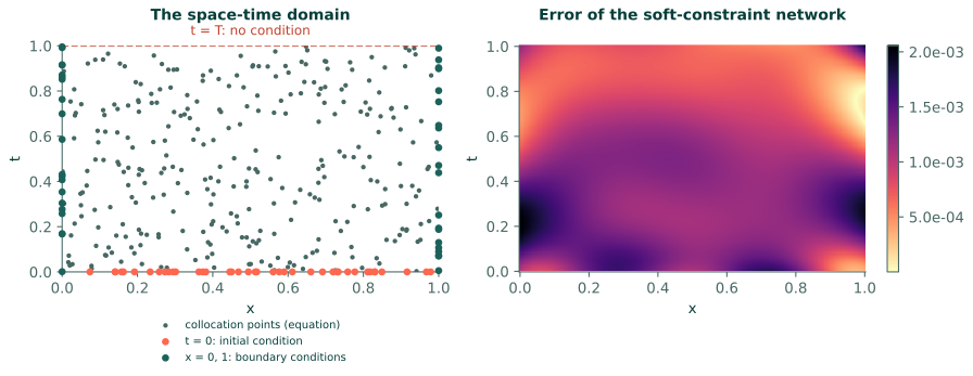
For one space dimension the region is a rectangle, $0 < x < 1$ by $0 < t < T$ (Figure 8.1). Each of its parts gets its own points and its own loss term:

• the interior gets collocation points, where the equation's residual is evaluated;
• the bottom face, $t = 0$, gets the initial condition;
• the side faces, $x = 0$ and $x = 1$ at every time, get the boundary conditions;
• the top face, $t = T$, gets nothing. Section 4.2 explained why: a condition at the final time instead of the initial one is the backward heat problem, which is ill-posed, and one at both ends would ask for more than the equation allows.

The heat equation, in thirty lines

The problem is $u_t = a\,u_{xx}$ with $a = 0.1$ on $0 < x < 1$, $0 < t < 1$, with $u = 0$ at both ends and $u(x, 0) = \sin(\pi x)$. Its solution is $u = e^{-a\pi^2 t}\sin(\pi x)$: the initial hump keeps its shape and decays, to 37% of its height by $t = 1$. Two versions are trained: one with the three conditions as loss terms (Section 6.3), and one with all three built into the trial function (Section 6.4),

$$u_\theta(x, t) = \sin(\pi x) + t\,x(1 - x)\,N_\theta(x, t),$$

which equals $\sin(\pi x)$ at $t = 0$ and zero at both ends, whatever the network outputs.

import math
import torch
import torch.nn as nn

def d(y, x):
    return torch.autograd.grad(y, x, torch.ones_like(y), create_graph=True)[0]

a = 0.1                                                     # the diffusivity
exact = lambda x, t: torch.exp(-a * math.pi**2 * t) * torch.sin(math.pi * x)

def train(hard, seed=0, epochs=5000):
    g = torch.Generator().manual_seed(seed)
    torch.manual_seed(seed)
    net = nn.Sequential(nn.Linear(2, 32), nn.Tanh(), nn.Linear(32, 32), nn.Tanh(),
                        nn.Linear(32, 32), nn.Tanh(), nn.Linear(32, 1))
    N = lambda x, t: net(torch.cat([2 * x - 1, 2 * t - 1], dim=1))        # both inputs scaled to [-1, 1]
    if hard:
        u = lambda x, t: torch.sin(math.pi * x) + t * x * (1 - x) * N(x, t)
    else:
        u = N
    x = torch.rand(1000, 1, generator=g).requires_grad_(True)              # collocation points in space-time
    t = torch.rand(1000, 1, generator=g).requires_grad_(True)
    x_0 = torch.rand(200, 1, generator=g)                                  # points on the face t = 0
    t_b = torch.rand(200, 1, generator=g)                                  # points on the faces x = 0, x = 1
    x_b = (torch.rand(200, 1, generator=g) < 0.5).float()
    opt = torch.optim.Adam(net.parameters(), lr=1e-3)
    for epoch in range(epochs):
        opt.zero_grad()
        u_c = u(x, t)
        r = (d(u_c, t) - a * d(d(u_c, x), x)) / (a * math.pi**2)         # divided by the natural decay rate
        loss = (r ** 2).mean()
        if not hard:
            loss = loss + ((u(x_0, torch.zeros_like(x_0)) - torch.sin(math.pi * x_0)) ** 2).mean() \
                        + (u(x_b, t_b) ** 2).mean()
        loss.backward()
        opt.step()
    return u

xs = torch.linspace(0, 1, 201).reshape(-1, 1)
print("largest error at time t, and in brackets as a fraction of the solution's height then")
print("          t = 0              0.25               0.5                0.75               1")
for hard in (False, True):
    u = train(hard)
    row = []
    for t_value in (0.0, 0.25, 0.5, 0.75, 1.0):
        ts = torch.full_like(xs, t_value)
        with torch.no_grad():
            err = (u(xs, ts) - exact(xs, ts)).abs().max().item()
        height = math.exp(-a * math.pi**2 * t_value)
        row.append(f"{err:.1e} ({err / height:.1e})")
    print(f"{'built in' if hard else 'soft':9s} " + "  ".join(row))

largest error at time t, and in brackets as a fraction of the solution's height then
          t = 0              0.25               0.5                0.75               1
soft      1.8e-03 (1.8e-03)  2.0e-03 (2.6e-03)  1.3e-03 (2.1e-03)  9.1e-04 (1.9e-03)  2.0e-03 (5.2e-03)
built in  0.0e+00 (0.0e+00)  8.7e-05 (1.1e-04)  6.8e-05 (1.1e-04)  9.6e-05 (2.0e-04)  4.1e-05 (1.1e-04)

Both versions work. The soft one keeps its largest error between about $10^{-3}$ and $2\times10^{-3}$ at every time, while the solution decays to 37% of its height, so as a fraction of the solution the error grows from 0.2% to 0.5% by $t = 1$. The loss counts errors in absolute terms, the same everywhere in space-time, so it has no reason to take more care where the solution is small (Exercise 2). With the three conditions built in, the error is twenty to fifty times smaller and stays near $10^{-4}$ of the solution's height throughout. The function the network must learn here, $N = (u - \sin\pi x)/\bigl(t\,x(1 - x)\bigr)$, lies between about $-4$ and $-2$ everywhere: gentle, which is the situation in which Section 6.4 found hard constraints helping.

Time is not like space

To the network, $t$ is one more input. To the equation it is not, in three ways that the rest of this chapter deals with.

1. Conditions sit on one side. Everything is fixed at $t = 0$ and nothing at $t = T$. In space, conditions usually surround the domain.
2. Causes come before effects. The solution at time $t$ depends only on earlier times. The loss does not know this: it weighs every part of space-time at once, and the optimiser is free to fit late times before early ones. Diffusion forgives this, because it smooths errors away as time goes on. Waves and transport carry errors forward instead, and over long times this becomes the main way PINNs fail: Section 8.2.
3. Time has its own scale. Diffusion over a length $L$ takes a time of order $L^2/a$, transport at speed $c$ a time $L/c$, an oscillation $1/\omega$. Measure time in that unit (Section 4.5) and choose the time window to match: a window much shorter than the natural time shows nothing happening, one much longer shows mostly the final state.

In the Studio

Tick Time dimension in the Domain block and set t initial and t final: the generated script then adds $t$ as the last input, scales it to $[-1, 1]$ with the space coordinates, and draws Initial points on the face $t = t_\text{initial}$ for the IC block. BC blocks apply on their faces at all times. The heat equation worked problem builds this example in the Studio. Building the initial condition into the trial function is a patch of the field function, exactly like Section 6.4's.

Exercises

1. For the wave equation $u_{tt} = c^2u_{xx}$ with $u(x, 0) = f(x)$ and $u_t(x, 0) = g(x)$, write a trial function that satisfies both initial conditions exactly.
2. In the soft run the error stayed near $10^{-3}$ while the solution decayed, so the error relative to the solution grew with time. Why does the loss behave like this, and what could you change if late times mattered most?
3. With $a = 0.1$ the natural decay rate $a\pi^2$ is about 1, so dividing the residual by it changes almost nothing. What would happen without that division if $a = 10^{-3}$, and what else should change?

Recap

• A PINN for an evolution equation takes $(x, t)$ and fits the whole history at once: the interior gets the equation, the face $t = 0$ the initial condition, the sides the boundary conditions, and the final time nothing.
• Initial conditions can be built into the trial function like boundary conditions; for the heat equation here that made the error ten times smaller.
• The loss treats all of space-time alike, without regard for cause and effect, and measures errors in absolute terms. Both matter more as the time window grows.