Forward and reverse mode

Section 3.4 computed the gradient of a loss by walking a computational graph backwards. That was one of two ways to organise the chain rule. This section builds both, each in about twenty lines of Python, so that nothing about torch.autograd is magic, and then measures why the backward one is what PINNs and neural networks use.

The computation as a graph

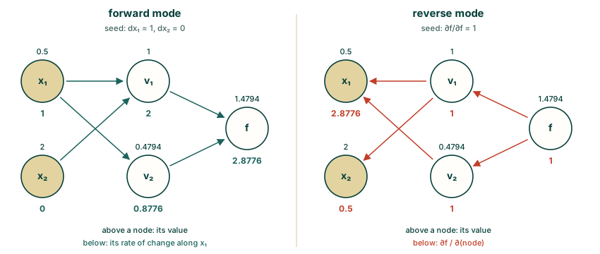
Take $f(x_1, x_2) = x_1x_2 + \sin x_1$. A program evaluates it as a sequence of elementary steps, each with an input or two and one output:

$$v_1 = x_1 x_2, \qquad v_2 = \sin x_1, \qquad f = v_1 + v_2.$$

Each step has local derivatives that are trivial to write down: $\partial v_1/\partial x_1 = x_2$, $\partial v_2/\partial x_1 = \cos x_1$, $\partial f/\partial v_1 = 1$, and so on. The chain rule combines them. The only question is the order.

Forward mode: carry a derivative along

Pick one input direction, say "increase $x_1$". Attach to every intermediate value a second number, its rate of change in that direction, written with a dot: $\dot x_1 = 1$, $\dot x_2 = 0$. Then push both numbers through each step together. For $v_1 = x_1x_2$ the product rule gives $\dot v_1 = \dot x_1 x_2 + x_1\dot x_2$; for $v_2 = \sin x_1$, $\dot v_2 = \cos(x_1)\,\dot x_1$. At the end $\dot f = \partial f/\partial x_1$.

The pair (value, rate) is called a dual number, and Python's operator overloading makes it a few lines. Wengert (1964) described this scheme in 1964, which makes automatic differentiation older than most of the programming languages it now runs in.

import math

class Dual:
    """A value together with its derivative in one chosen direction."""
    def __init__(self, val, dot=0.0):
        self.val, self.dot = val, dot
    def __add__(self, o):
        o = o if isinstance(o, Dual) else Dual(o)
        return Dual(self.val + o.val, self.dot + o.dot)
    def __mul__(self, o):
        o = o if isinstance(o, Dual) else Dual(o)
        return Dual(self.val * o.val, self.dot * o.val + self.val * o.dot)     # the product rule
    __radd__, __rmul__ = __add__, __mul__

def sin(d):  return Dual(math.sin(d.val), math.cos(d.val) * d.dot)                 # the chain rule, once each
def exp(d):  return Dual(math.exp(d.val), math.exp(d.val) * d.dot)
def tanh(d): return Dual(math.tanh(d.val), (1 - math.tanh(d.val) ** 2) * d.dot)

f = lambda x: x * sin(x) + exp(tanh(x))
out = f(Dual(0.7, 1.0))                     # value 0.7, direction 1: "d/dx"
by_hand = math.sin(0.7) + 0.7 * math.cos(0.7) + math.exp(math.tanh(0.7)) * (1 - math.tanh(0.7) ** 2)
print(f"f(0.7) = {out.val:.12f}   f'(0.7): dual numbers {out.dot:.12f},  by hand {by_hand:.12f}")

f(0.7) = 2.281047196305   f'(0.7): dual numbers 2.341240850991,  by hand 2.341240850991

The function f was written for ordinary numbers and never mentions derivatives. Handed a dual number, it returns its derivative as a by-product, exact to the last digit. The price is that one pass gives the derivative in one input direction. For a function of $n$ inputs, the full gradient takes $n$ passes.

Reverse mode: send sensitivities back

Reverse mode runs the program once, forwards, recording each step and its local derivatives. Then it walks the record backwards from the output, carrying for every value the sensitivity of the output to it, written with a bar: $\bar f = 1$, then $\bar v_1 = \bar f\cdot 1$, $\bar v_2 = \bar f\cdot1$, and $\bar x_1 = \bar v_1 x_2 + \bar v_2\cos x_1$, which collects contributions from every path through $x_1$. This is exactly the backward pass of Section 3.4, and one sweep gives the derivative of the output with respect to every input at once. A record that can do this is called a tape:

class Var:
    """A value that remembers what it was computed from, and the local slope to each parent."""
    def __init__(self, val, parents=()):
        self.val, self.parents, self.grad = val, parents, 0.0
    def __add__(self, o): return Var(self.val + o.val, [(self, 1.0), (o, 1.0)])
    def __mul__(self, o): return Var(self.val * o.val, [(self, o.val), (o, self.val)])
    def backward(self):
        order, seen = [], set()
        def visit(v):                          # every value after the ones it depends on
            if id(v) not in seen:
                seen.add(id(v))
                for p, _ in v.parents:
                    visit(p)
                order.append(v)
        visit(self)
        self.grad = 1.0
        for v in reversed(order):              # outputs first: hand each sensitivity to the parents
            for p, local in v.parents:
                p.grad += local * v.grad

def vsin(v): return Var(math.sin(v.val), [(v, math.cos(v.val))])

x1, x2, x3 = Var(0.5), Var(2.0), Var(-1.0)
g = x1 * x2 + vsin(x3) * x1
g.backward()
print(f"g = {g.val:.6f}   one backward sweep: ({x1.grad:.6f}, {x2.grad:.6f}, {x3.grad:.6f})")
print(f"by hand:                      ({2.0 + math.sin(-1.0):.6f}, {0.5:.6f}, {0.5 * math.cos(-1.0):.6f})")

g = 0.579265   one backward sweep: (1.158529, 0.500000, 0.270151)
by hand:                      (1.158529, 0.500000, 0.270151)

Three partial derivatives from one backward sweep. The cost is memory: the tape must keep every intermediate value until the sweep is over, which is why training a network uses far more memory than evaluating it. torch.autograd is this idea, written in C++ and extended to tensors. Figure 5.2 draws the two modes on the example above.

Which mode when

For a function with $n$ inputs and $m$ outputs, forward mode needs $n$ passes for the full matrix of derivatives (the Jacobian) and reverse mode needs $m$. Training has one output, the loss, and thousands of inputs, the weights: reverse mode wins by a factor of thousands. PyTorch offers both through torch.func, so the difference can be timed on a function of 500 inputs:

import time
import torch
from torch.func import jvp, grad

torch.manual_seed(0)
n = 500
W1, W2 = torch.randn(200, n) / n**0.5, torch.randn(1, 200) / 200**0.5
F = lambda x: (W2 @ torch.tanh(W1 @ x)).sum()          # 500 inputs, one output
x = torch.randn(n)

forward_mode = lambda x: torch.stack([jvp(F, (x,), (e,))[1] for e in torch.eye(n)])   # n passes
reverse_mode = lambda x: grad(F)(x)                                                    # one backward sweep

print(f"the two gradients differ by at most {(forward_mode(x) - reverse_mode(x)).abs().max():.0e}")

def best_time(fn, reps):
    times = []
    for _ in range(reps):
        t0 = time.perf_counter(); fn(x); times.append(time.perf_counter() - t0)
    return min(times)

t_fwd, t_rev = best_time(forward_mode, 3), best_time(reverse_mode, 20)
print(f"forward mode {t_fwd * 1e3:.0f} ms, reverse mode {t_rev * 1e3:.2f} ms: about {t_fwd / t_rev:.0f} times slower")

the two gradients differ by at most 3e-08
forward mode 106 ms, reverse mode 0.15 ms: about 695 times slower

Same numbers, to the rounding of 32-bit arithmetic; a very different bill. The exact times depend on your machine, and part of the forward-mode cost here is Python looping over 500 directions, but the factor of order $n$ is the point.

Exercises

1. Push the dual number $x = 2 + 1\varepsilon$ through $f(x) = x^3$ by repeated multiplication, using $\varepsilon^2 = 0$. What do you get, and why is it $f'(2)$?
2. For $f(x_1, x_2) = x_1x_2 + \sin x_1$, how many forward-mode passes give the full gradient? How many reverse-mode sweeps?
3. A function maps one number to a vector of 1000 numbers, such as a trajectory computed from one initial velocity. Which mode gives all 1000 derivatives in one pass?

Recap

• Automatic differentiation applies the chain rule to a recorded sequence of elementary steps, with numbers, not formulas.
• Forward mode carries one directional derivative along with the values; reverse mode records a tape and sweeps it backwards, getting the derivative with respect to every input in one go, at the cost of memory.
• Choose by shape: $n$ inputs and $m$ outputs cost $n$ forward passes or $m$ reverse sweeps. Training a network is the extreme case for reverse mode.

References

- Wengert, R. E. (1964). A simple automatic derivative evaluation program. Communications of the ACM, 7(8), 463–464. doi:10.1145/355586.364791