Long times and causality

Section 6.2 solved an oscillator over two periods. This section asks for more periods of the same motion, and finds the way PINNs most often fail on evolution problems. Krishnapriyan et al. (2021) describe the same failure for transport (the advection equation) and for reaction and diffusion problems; an oscillator is the smallest problem that shows it, and it runs in a few minutes.

The experiment

An undamped oscillator, $u'' + \omega^2 u = 0$ with $\omega = 2\pi$, $u(0) = 1$ and $u'(0) = 0$, whose solution $\cos(2\pi t)$ completes one period per second. The training function is Section 6.2's, scaled the same way, for a time window $[t_\text{start}, t_\text{end}]$ and any starting value and velocity, with 100 collocation points per second spread evenly in the manner of a Latin hypercube (Section 7.1):

import math
import torch
import torch.nn as nn

def d(y, t):
    return torch.autograd.grad(y, t, torch.ones_like(y), create_graph=True)[0]

omega = 2 * math.pi                                         # one period per second
exact = lambda t: torch.cos(omega * t)

def train(t_start, t_end, u_start=1.0, v_start=0.0, seed=0, epochs=10000):
    """A PINN for u'' + omega^2 u = 0 on [t_start, t_end], given u and u' at t_start."""
    torch.manual_seed(seed)
    net = nn.Sequential(nn.Linear(1, 32), nn.Tanh(), nn.Linear(32, 32), nn.Tanh(),
                        nn.Linear(32, 32), nn.Tanh(), nn.Linear(32, 1))
    u = lambda t: net(2 * (t - t_start) / (t_end - t_start) - 1)
    n = round(100 * (t_end - t_start))                     # 100 points per second, one in each slice
    t_col = (t_start + (t_end - t_start) * (torch.arange(n).reshape(-1, 1) + torch.rand(n, 1)) / n).requires_grad_(True)
    t_0 = torch.full((1, 1), float(t_start), requires_grad=True)
    opt = torch.optim.Adam(net.parameters(), lr=1e-3)
    for epoch in range(epochs):
        opt.zero_grad()
        u_c = u(t_col)
        r = (d(d(u_c, t_col), t_col) + omega**2 * u_c) / omega**2
        u0 = u(t_0)
        v0 = d(u0, t_0) / omega
        loss = (r ** 2).mean() + ((u0 - u_start) ** 2).sum() + ((v0 - v_start / omega) ** 2).sum()
        loss.backward()
        opt.step()
    return u

for T in (2, 5, 10):
    u = train(0, T)
    t = torch.linspace(0, T, 2001).reshape(-1, 1)
    with torch.no_grad():
        err = ((u(t) - exact(t)).norm() / exact(t).norm()).item()
        peaks = [u(t[(t[:, 0] >= s) & (t[:, 0] <= s + 1)]).abs().max().item() for s in range(T)]
    print(f"{T:2d} periods: relative L2 error {err:.1e};  largest |u| in each second: "
          + " ".join(f"{p:.2f}" for p in peaks))

 2 periods: relative L2 error 3.5e-03;  largest |u| in each second: 1.00 1.00
 5 periods: relative L2 error 7.6e-01;  largest |u| in each second: 1.00 0.67 0.37 0.08 0.02
10 periods: relative L2 error 9.1e-01;  largest |u| in each second: 1.00 0.60 0.24 0.02 0.01 0.00 0.00 0.00 0.00 0.00

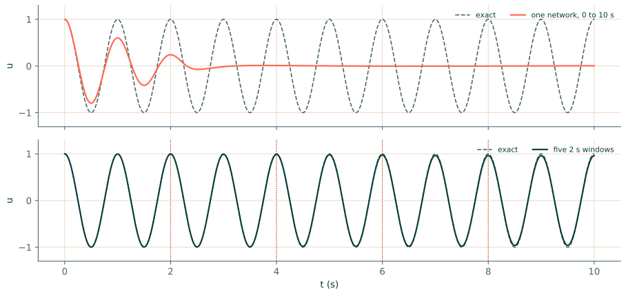
Over two periods the PINN is as good as Section 6.2's. Over five and ten it fails, and the last columns show how: the oscillation starts at full height and fades, to a third or a quarter of it in the third second and to almost nothing by the fourth. Wherever the network is close to zero, which is most of the window, it satisfies the equation; at the start it satisfies the initial conditions; only the fading in between is wrong. Figure 8.2 (top) shows the ten-period run.

Why the zero function wins

Section 6.2's first attempt converged to $u \approx 0$ because the residual was badly scaled. Here the residual is scaled correctly, and the zero function wins anyway. Three facts combine.

• Zero satisfies the equation. $u = 0$ makes the residual vanish everywhere. It fails only the initial conditions.
• A function that follows the start and then fades away is cheap. It satisfies the initial conditions and the equation everywhere except where it fades. The loss averages the residual over all the collocation points, so the fading region's cost is diluted by the length of the window: the longer the window, the cheaper the wrong answer.
• Information travels by gradient descent. The only way the network learns what happens at $t = 5$ is through the chain of residuals linking it to $t = 0$. In a time-stepping solver each step hands the state to the next. In a PINN all times are trained at once, the late times settle on whatever satisfies the equation locally, and zero does, long before the correct oscillation has been passed along to them.

The result breaks causality: the network fits the late times before it has got the early ones right, the opposite of the order in which the physics determines them. Wang et al. (2024) name the failure this way, and Daw et al. (2023) call it a propagation failure, the correct solution not spreading from the initial and boundary conditions into the domain. For transport, the failure appears as the speed rises (Krishnapriyan et al., 2021): more of the solution has to be passed along in the same time.

A fix: one window at a time

The remedy closest to classical solvers is time marching: split the time interval into windows short enough for a PINN to handle, train a network on the first window, and use its value and velocity at the end as the initial conditions of the next window (Mattey & Ghosh, 2022; Krishnapriyan et al., 2021). Here, five windows of 2 seconds, each exactly the problem that worked:

pieces, u_start, v_start = [], 1.0, 0.0
for t_start in range(0, 10, 2):
    u = train(t_start, t_start + 2, u_start, v_start)
    t_end = torch.full((1, 1), t_start + 2.0, requires_grad=True)
    u_end = u(t_end)
    u_start, v_start = u_end.item(), d(u_end, t_end).item()     # hand the state over to the next window
    pieces.append(u)

errors, squared, total = [], 0.0, 0.0
for i, u in enumerate(pieces):
    t = torch.linspace(2 * i, 2 * i + 2, 401).reshape(-1, 1)
    with torch.no_grad():
        e = u(t) - exact(t)
    errors.append((e.norm() / exact(t).norm()).item())
    squared, total = squared + e.pow(2).sum().item(), total + exact(t).pow(2).sum().item()
print("error in each window:", "  ".join(f"{e:.1e}" for e in errors))
print(f"over all 10 periods: {math.sqrt(squared / total):.1e}")

error in each window: 3.5e-03  8.6e-03  1.7e-02  2.8e-02  3.9e-02
over all 10 periods: 2.3e-02

Every window is now accurate to a few per cent or better, and the whole ten periods to 2%, against 91% for a single network (Figure 8.2, bottom). The error grows from window to window: each window starts from its predecessor's final value and velocity, which are slightly wrong, and an oscillator carries a wrong start forward as an error of phase and amplitude. Every time-stepping method pays this price; it is mild here, and smaller the more accurately each window is trained. The other cost is five training runs instead of one.

Other fixes

Time marching costs one training run per window and gives up one advantage of a PINN, a single network for all times. The alternatives keep one network and change how it is trained.

• Causal weighting (Wang et al., 2024) splits time into slices and multiplies the residual loss of slice $i$ by $$w_i = \exp\Bigl(-\varepsilon \sum_{k < i} L_k\Bigr),$$ where $L_k$ is the mean squared residual of an earlier slice $k$, and the weights are held fixed while the gradient is taken. A slice's residual counts only once every slice before it is small: the loss itself respects cause and effect. The tolerance $\varepsilon$ needs tuning, and the authors raise it in steps during training. In their examples the weights are combined with a modified network architecture and, for periodic problems, with Fourier features of the inputs (Chapter 11).
• A curriculum (Krishnapriyan et al., 2021) trains on an easy version first, such as a slow transport speed or a short window, and makes it harder step by step, starting each stage from the previous weights.
• Resampling towards the trouble (Section 7.2), with R3 sampling (Daw et al., 2023) designed for exactly this failure.

None of them is free, and none is needed for a problem like Section 8.1's heat equation, which forgives the order in which it is learnt.

Exercises

1. In the 10-period run, the largest $|u|$ falls towards zero after the first few periods. Predict what a run on $[0, 10]$ with the weight of the initial-condition terms raised to 100 would do, and why it is not a cure.
2. Time marching hands over $u$ and $u'$ at each window boundary. What goes wrong if it hands over only $u$?
3. How would you march in time for the heat equation of Section 8.1, where the state is a whole function of $x$?

Recap

• Over long times a PINN can fit the late times before the early ones and settle on a solution of the equation that ignores the initial conditions, often zero. The longer the window, the cheaper this wrong answer.
• Time marching restores the order of cause and effect by training one short window after another, handing over the full state at each boundary.
• Causal weighting, curricula and residual-based resampling keep a single network; they need tuning, and the hardest problems need them combined with a better network.

References

- Daw, A., Bu, J., Wang, S., Perdikaris, P., & Karpatne, A. (2023). Mitigating propagation failures in physics-informed neural networks using retain-resample-release (R3) sampling. Proceedings of the 40th International Conference on Machine Learning, 202, 7264–7302. https://proceedings.mlr.press/v202/daw23a.html
- Krishnapriyan, A. S., Gholami, A., Zhe, S., Kirby, R. M., & Mahoney, M. W. (2021). Characterizing possible failure modes in physics-informed neural networks. Advances in Neural Information Processing Systems, 34, 26548–26560. https://proceedings.neurips.cc/paper_files/paper/2021/hash/df438e5206f31600e6ae4af72f2725f1-Abstract.html
- Mattey, R., & Ghosh, S. (2022). A novel sequential method to train physics informed neural networks for Allen Cahn and Cahn Hilliard equations. Computer Methods in Applied Mechanics and Engineering, 390, 114474. doi:10.1016/j.cma.2021.114474
- Wang, S., Sankaran, S., & Perdikaris, P. (2024). Respecting causality for training physics-informed neural networks. Computer Methods in Applied Mechanics and Engineering, 421, 116813. doi:10.1016/j.cma.2024.116813