Inverse problems

Every problem so far was forward: the equation, its coefficients and its conditions were known, and the PINN found the solution. In an inverse problem part of the equation is unknown (a material property, a source, a boundary condition) and measurements of the solution are available instead. The classical approach nests two loops: guess the coefficient, solve the forward problem, compare with the measurements, improve the guess, and solve again. A PINN does both at once. The unknown coefficient becomes one more trainable parameter, next to the weights, and the measurements become one more term in the loss. Inverse problems were part of the PINN idea from the start (Raissi et al., 2019); its best-known demonstration recovered the velocity and pressure of a flow from measurements of a dye carried by it (Raissi et al. (2020)).

The problem

A rod's ends are held at temperature zero, and its diffusivity $a$ is unknown. Five thermometers, at $x = 0.1, 0.3, \dots, 0.9$, are read every 0.05 s from $t = 0$ to $t = 1$: 105 readings in all. The initial temperature is not given to the PINN, only the readings. Behind the scenes the readings come from $a = 0.1$ and

$$u(x, t) = e^{-a\pi^2 t}\sin(\pi x) + \tfrac12\,e^{-4a\pi^2 t}\sin(2\pi x),$$

a hump and a two-lobed wave that decays four times faster. The loss has three terms: the residual of $u_t = a\,u_{xx}$ at collocation points, the mismatch with the readings, and the boundary condition:

$$L(\theta, a) = \frac{1}{N_r}\sum_{i} r_\theta(x_i, t_i; a)^2 + \frac{1}{N_d}\sum_{j}\bigl(u_\theta(x_j, t_j) - d_j\bigr)^2 + \frac{1}{N_b}\sum_k u_\theta(x_k, t_k)^2.$$

The unknown is stored as its logarithm, $a = e^{s}$ with $s$ trained. That keeps $a$ positive whatever the optimiser does, and makes every step a relative change: a step that changes $a$ by 1% does so whether $a$ is 1 or 0.01. Like the corner coefficient of Section 7.3, it gets its own, larger learning rate. The training starts from $a = 1$, ten times too large.

import math
import numpy as np
import torch
import torch.nn as nn

def d(y, x):
    return torch.autograd.grad(y, x, torch.ones_like(y), create_graph=True)[0]

a_true = 0.1                                        # used only to make the readings
truth = lambda x, t: (torch.exp(-a_true * math.pi**2 * t) * torch.sin(math.pi * x)
                      + 0.5 * torch.exp(-4 * a_true * math.pi**2 * t) * torch.sin(2 * math.pi * x))

X, T = torch.meshgrid(torch.tensor([0.1, 0.3, 0.5, 0.7, 0.9]), torch.linspace(0, 1, 21), indexing="ij")
x_d, t_d = X.reshape(-1, 1), T.reshape(-1, 1)       # five thermometers, 21 readings each
u_d = truth(x_d, t_d)

def train_inverse(u_d, x_d=x_d, t_d=t_d, a_start=1.0, seed=0, epochs=5000):
    g = torch.Generator().manual_seed(seed)
    torch.manual_seed(seed)
    net = nn.Sequential(nn.Linear(2, 32), nn.Tanh(), nn.Linear(32, 32), nn.Tanh(),
                        nn.Linear(32, 32), nn.Tanh(), nn.Linear(32, 1))
    u = lambda x, t: net(torch.cat([2 * x - 1, 2 * t - 1], dim=1))
    log_a = torch.tensor([math.log(a_start)], requires_grad=True)     # the unknown, as a logarithm
    x = torch.rand(1000, 1, generator=g).requires_grad_(True)
    t = torch.rand(1000, 1, generator=g).requires_grad_(True)
    t_b = torch.rand(200, 1, generator=g)
    x_b = (torch.rand(200, 1, generator=g) < 0.5).float()
    opt = torch.optim.Adam([{"params": net.parameters()}, {"params": [log_a], "lr": 1e-2}], lr=1e-3)
    history = []
    for epoch in range(1, epochs + 1):
        opt.zero_grad()
        u_c = u(x, t)
        r = d(u_c, t) - log_a.exp() * d(d(u_c, x), x)                 # the equation, with a unknown
        loss = (r ** 2).mean() + ((u(x_d, t_d) - u_d) ** 2).mean() + (u(x_b, t_b) ** 2).mean()
        loss.backward()
        opt.step()
        if epoch % 1000 == 0:
            history.append(log_a.exp().item())
    return u, history

u, history = train_inverse(u_d, epochs=10000)
print("estimate of a after every 1000 epochs:")
print("  ".join(f"{a:.4f}" for a in history))

estimate of a after every 1000 epochs:
0.0912  0.0970  0.0985  0.0991  0.0992  0.0994  0.0994  0.0997  0.0997  0.0998

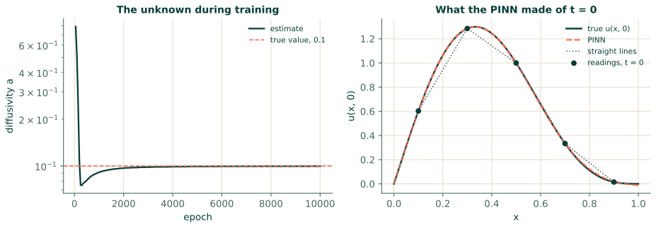
From a starting value ten times too large, the estimate is within 10% of the truth after 1000 epochs, within 1% after 4000, and ends at 0.0998, 0.2% from the true 0.1. It approaches from below and keeps creeping up as the network's fit to the field improves: the estimate of $a$ is only as good as the network's picture of the temperature, and the two improve together.

What the equation adds

The network was never told the initial temperature. It has five readings at $t = 0$, and the equation, which links those readings to the hundred others. Compare its reconstruction of $u(x, 0)$ with the best one can do from the five readings at $t = 0$ alone, straight lines between them and the zero ends:

xs = torch.linspace(0, 1, 201).reshape(-1, 1)
true_0 = truth(xs, torch.zeros_like(xs)).flatten()
with torch.no_grad():
    pinn_0 = u(xs, torch.zeros_like(xs)).flatten()
x_known = np.array([0.0, 0.1, 0.3, 0.5, 0.7, 0.9, 1.0])
u_known = truth(torch.tensor(x_known).reshape(-1, 1), torch.zeros(7, 1)).flatten().numpy()
lines_0 = torch.tensor(np.interp(xs.flatten().numpy(), x_known, u_known))
print(f"largest error in the initial temperature:  PINN {(pinn_0 - true_0).abs().max():.1e}"
      f"   straight lines between the readings {(lines_0 - true_0).abs().max():.1e}")

largest error in the initial temperature:  PINN 1.2e-02   straight lines between the readings 1.2e-01

The PINN's initial temperature is ten times more accurate than straight lines through the readings. The straight lines use only the five readings at $t = 0$. The PINN also uses the hundred later ones, because the equation says how a temperature profile evolves, so later readings carry information about the profile at $t = 0$ between the thermometers. That is the general strength of the method for inverse problems: the equation is a model of what happens in the gaps between measurements.

Practical points

• Scale the unknown. Train its logarithm, or write it as a known reference value times a factor near 1, so that its steps are relative and of a sensible size.
• Balance the terms. The data term and the residual pull in different directions when either is imperfect. Here both are of order one by construction; when they are not, their weights matter as much as in Chapter 10.
• An unknown function is a second network. A diffusivity that varies along the rod, $a(x)$, is the output of a second small network (or a second output of the first), trained with everything else.
• Check what the data can determine before trusting an estimate, especially with noise: the subject of the next section.

In the Studio

The Studio has no data term and no trainable coefficients yet, but a generated script takes both in a dozen lines. For the 1D Poisson script, here is the source strength $s$ in $u'' = -s\,\pi^2\sin(\pi x)$ treated as unknown and recovered from four readings:

# not run
import math
import torch
import poisson_1d as p                                   # the generated script, saved as poisson_1d.py

log_s = torch.nn.Parameter(torch.tensor([math.log(3.0)]))   # unknown source strength, first guess 3
x_data = torch.tensor([[0.2], [0.4], [0.6], [0.8]])          # sensor positions...
u_data = torch.sin(math.pi * x_data)                         # ...and their readings

def residual_pde1(pts):                                  # the generated residual, with s in front of the source
    u = p.field(pts, 0)
    u_xx = p.grad_of(p.grad_of(u, pts)[:, 0:1], pts)[:, 0:1]
    return u_xx + log_s.exp() * math.pi**2 * torch.sin(math.pi * pts[:, 0:1])

generated_terms = p.loss_terms
def loss_terms(pts):
    terms = generated_terms(pts)
    terms["data"] = ((p.field(x_data) - u_data) ** 2).mean()  # logged and plotted like the other terms
    return terms

p.residual_pde1, p.loss_terms = residual_pde1, loss_terms
p.build_optimiser = lambda lr=p.LEARNING_RATE: torch.optim.Adam(
    [{"params": p.net.parameters()}, {"params": [log_s], "lr": 1e-2}], lr=lr)
p.TERM_SCALES["data"] = 100.0                           # see below
history = p.train()
print("s =", log_s.exp().item())

total_loss in the generated script weighs every term it finds, so the new data term is trained, logged and plotted like the others, and train builds its optimiser through build_optimiser, which now includes $s$. The weight on the last line matters. The generated residual is unscaled, of natural size $\pi^2 \approx 10$ (Section 4.5), and four readings carry little weight against it: without that line, the script's 5000 epochs end at $s = 1.07$, from a first guess of 3; with it, at $s = 1.000$.

Exercises

1. Why does the inverse problem above need no initial condition, when the forward problem of Section 8.1 could not do without one?
2. Suppose the unknown were stored directly as $a$ and trained with a learning rate of $10^{-2}$, starting from 1. What could go wrong on the way to 0.1?
3. A colleague proposes to recover $a$ by fitting the readings with a plain network, with no residual term, and then computing $u_t/u_{xx}$ from it at the sensors. Why is this likely to give a poor estimate?

Recap

• An inverse problem makes the unknown a trainable parameter and adds a data term to the loss; the forward and inverse problems are solved together, in one training run.
• Train the logarithm of a positive unknown, with its own learning rate.
• The equation fills the gaps between the measurements: here it recovered the unseen initial temperature far better than the readings alone could.

References

- Raissi, M., Perdikaris, P., & Karniadakis, G. E. (2019). Physics-informed neural networks: A deep learning framework for solving forward and inverse problems involving nonlinear partial differential equations. Journal of Computational Physics, 378, 686–707. doi:10.1016/j.jcp.2018.10.045
- Raissi, M., Yazdani, A., & Karniadakis, G. E. (2020). Hidden fluid mechanics: Learning velocity and pressure fields from flow visualizations. Science, 367(6481), 1026–1030. doi:10.1126/science.aaw4741