Elliptic, parabolic, hyperbolic
Second-order PDEs come in three families. The family tells you how information travels through the domain, which conditions the problem needs, and where a PINN is likely to struggle.
Laplace's equation, the heat equation and the wave equation look alike on paper: each has two second derivatives, or one second and one first. They behave completely differently. Heat smooths and forgets, waves travel and remember, and the steady temperature of a plate depends on every point of its edge at once. The difference can be read off the coefficients of the equation, and it is worth knowing before you train anything.
The test
Write a linear second-order PDE in two variables $x$ and $y$ (one of them may be time) as
$$A\,u_{xx} + 2B\,u_{xy} + C\,u_{yy} + (\text{terms with first derivatives or none}) = 0.$$
Only the second-order part decides the family, through the sign of $B^2 - AC$:
| $B^2 - AC$ | Family | Prototype |
|---|---|---|
| $< 0$ | elliptic | Laplace, $u_{xx} + u_{yy} = 0$ |
| $= 0$ | parabolic | heat, $a\,u_{xx} - u_t = 0$ |
| $> 0$ | hyperbolic | wave, $c^2 u_{xx} - u_{tt} = 0$ |
The names come from the conic sections $Ax^2 + 2Bxy + Cy^2 = 1$, which are ellipses, parabolas or hyperbolas by the same test (Strauss, 2008, sec. 1.6). A few lines of code apply it:
import numpy as np

def classify(A, B, C):
    """A u_xx + 2B u_xy + C u_yy + (lower-order terms) = 0."""
    d = B**2 - A * C
    return "elliptic" if d < 0 else ("parabolic" if d == 0 else "hyperbolic")

cases = {
    "Laplace     u_xx + u_yy = 0":            (1, 0, 1),
    "heat        a u_xx - u_t = 0    (y = t)": (0.1, 0, 0),
    "wave        c^2 u_xx - u_tt = 0 (y = t)": (1, 0, -1),
    "            u_xx + 4 u_xy + u_yy = 0":   (1, 2, 1),
    "Burgers     nu u_xx - u_t - u u_x = 0":  (0.01, 0, 0),
}
for name, (A, B, C) in cases.items():
    print(f"{name:42s} B^2 - AC = {B*B - A*C:+5.2f}  ->  {classify(A, B, C)}")
Laplace     u_xx + u_yy = 0                B^2 - AC = -1.00  ->  elliptic
heat        a u_xx - u_t = 0    (y = t)    B^2 - AC = +0.00  ->  parabolic
wave        c^2 u_xx - u_tt = 0 (y = t)    B^2 - AC = +1.00  ->  hyperbolic
            u_xx + 4 u_xy + u_yy = 0       B^2 - AC = +3.00  ->  hyperbolic
Burgers     nu u_xx - u_t - u u_x = 0      B^2 - AC = +0.00  ->  parabolic
Two rows deserve a comment. The fourth looks like Laplace's equation with an extra term, but the mixed derivative is large enough to make it a wave equation in disguise: a rotation of the axes turns it into $3u_{\xi\xi} - u_{\eta\eta} = 0$. And Burgers' equation, $u_t + u\,u_x = \nu\,u_{xx}$, is parabolic whenever the viscosity $\nu$ is positive, because its only second derivative is $\nu\,u_{xx}$. The nonlinear term is first order and does not enter the test. Only with $\nu = 0$ does it become the inviscid Burgers equation, a first-order hyperbolic one.
Burgers in the Studio
The Studio's Equation type menu lists Burgers under Hyperbolic. That grouping describes how the equation behaves when $\nu$ is small, as in Section 13.6: away from the shock it carries information along like a wave. Strictly, with any viscosity at all, it is parabolic. Both classes need the same conditions (boundary values and one initial condition), so nothing you enter changes.
Equations whose coefficients vary can change family from place to place. The Tricomi equation $y\,u_{xx} + u_{yy} = 0$, a model of flow past the speed of sound, has $B^2 - AC = -y$: elliptic above the line $y = 0$ and hyperbolic below it.
What each family means
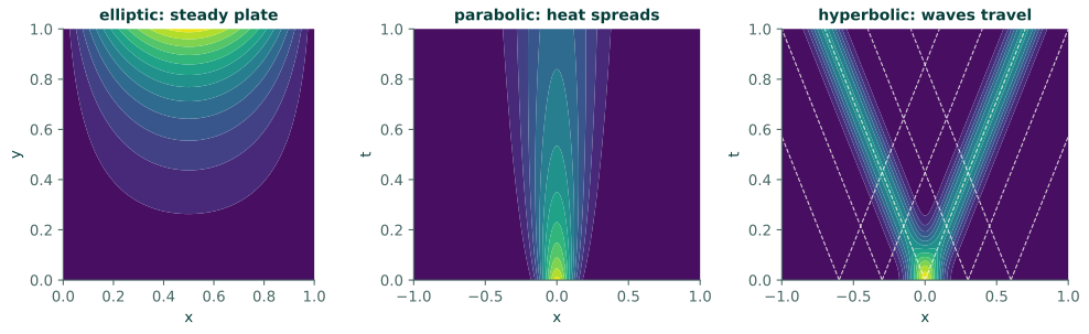
Elliptic equations describe equilibrium. There is no time. The value at any interior point depends on the data on the whole boundary, and the solution is as smooth as the coefficients allow: the solution of Laplace's equation is, at every point, the average of its values on any circle around that point. Such a problem needs one condition on every part of a closed boundary, and no initial condition.
Parabolic equations describe diffusion. They smooth: sharp features in the initial data disappear at once, fine ones fastest (Section 4.2). Any disturbance is felt everywhere immediately, although very weakly far away. They need an initial condition and boundary conditions, and they are well posed forward in time only.
Hyperbolic equations describe waves and transport. Information travels at a finite speed along curves called characteristics. For the wave equation they are the lines $x \pm ct = \text{constant}$, and a disturbance cannot reach a point before the time its distance divided by $c$. Sharp features are carried along, not smoothed, and nonlinear equations can create new ones: shocks.
The difference in propagation speed is easy to see in numbers. Start both the heat equation (diffusivity $a = 1$) and the wave equation (speed $c = 1$) from the same box of height 1 on $|x| < 0.1$, on an infinite line, where both have exact solutions, and look at three places a little later:
from scipy.special import erfc

a, c, w = 1.0, 1.0, 0.1           # diffusivity, wave speed, half-width of the initial box
heat = lambda x, t: 0.5 * (erfc((x - w) / np.sqrt(4 * a * t)) - erfc((x + w) / np.sqrt(4 * a * t)))
box = lambda x: (np.abs(x) < w).astype(float)
wave = lambda x, t: 0.5 * (box(x - c * t) + box(x + c * t))     # d'Alembert's formula, released from rest

print("    t      x     heat u(x, t)    wave u(x, t)")
for t in [0.01, 0.1, 0.5]:
    for x in [0.25, 0.5, 1.0]:
        print(f"{t:5.2f}  {x:5.2f}   {heat(x, t):13.3e}   {wave(x, t):13.3e}")
    t      x     heat u(x, t)    wave u(x, t)
 0.01   0.25       1.378e-01       0.000e+00
 0.01   0.50       2.328e-03       0.000e+00
 0.01   1.00       9.830e-11       0.000e+00
 0.10   0.25       1.517e-01       0.000e+00
 0.10   0.50       9.569e-02       0.000e+00
 0.10   1.00       1.513e-02       0.000e+00
 0.50   0.25       7.721e-02       0.000e+00
 0.50   0.50       7.033e-02       5.000e-01
 0.50   1.00       4.839e-02       0.000e+00
The heat solution is positive at every point at every positive time: at $t = 0.01$ it has already reached $x = 1$, at a level of about $10^{-10}$. The wave solution is exactly zero until the front arrives, at $t = (x - 0.1)/c$, carries the full half-height of the box while the pulse passes, and is zero again afterwards: at $t = 0.5$ the pulse has already gone by $x = 0.25$ and not yet reached $x = 1$. Figure 4.3 shows the three behaviours side by side.
What it means for a PINN
A PINN minimises the residual everywhere at once, in space and time together, with no notion of which way information is supposed to flow. That suits some families better than others.
- Elliptic problems are usually the friendliest: the solution is smooth and every point is coupled to every other, which is how a PINN treats them anyway. The Poisson and Laplace problems in Chapter 13 are of this kind.
- Parabolic problems are usually fine while the solution stays smooth, as in Section 13.3. Trouble starts where the data are sharp or disagree at a corner (Section 4.2).
- Hyperbolic problems, and parabolic ones with little diffusion, are the hard ones. Their residual can be small for functions that ignore the initial condition, and sharp fronts need a network with enough capacity to bend quickly. Section 8.2 shows a PINN failing in exactly this way when an oscillation is followed for many periods, and what helps.
Exercises
- Classify (a) $u_{xx} - 4u_{xy} + 4u_{yy} = 0$; (b) $u_t = u_{xx} + u_x$; (c) $u_{xx} + y\,u_{yy} = 0$ in the region $y > 0$.
- The advection equation $u_t + c\,u_x = 0$ is first order. Along which lines in the $(x, t)$ plane is $u$ constant? On $0 \le x \le 1$ with $c > 0$, at which end does it need a boundary condition?
- Why does the heat equation need no condition at the final time $t = T$?
Answers
- (a) $A = 1$, $2B = -4$ so $B = -2$, $C = 4$: $B^2 - AC = 4 - 4 = 0$, parabolic. (b) Only $u_{xx}$ is second order: parabolic. (c) $B^2 - AC = -y < 0$: elliptic.
- Along the characteristics $x - ct = \text{constant}$, because $u = g(x - ct)$ (Section 4.1, Exercise 2). With $c > 0$ they move to the right, so information enters at $x = 0$: that end needs a condition (the inflow), and $x = 1$ must be left free.
- The equation is first order in time and propagates information forward. The initial condition and the boundary values determine the solution at all later times, including $t = T$; imposing a value there as well would over-determine the problem.
Recap
- The sign of $B^2 - AC$ in the second-order part classifies a PDE: elliptic (negative), parabolic (zero), hyperbolic (positive). Viscous Burgers is parabolic; only the inviscid equation is hyperbolic.
- Elliptic means equilibrium and global coupling; parabolic means smoothing and infinite speed; hyperbolic means finite speed along characteristics, and sharp features that persist or form.
- A PINN treats every point alike, which suits elliptic problems best and hyperbolic or advection-dominated problems worst.
References
- Strauss, W. A. (2008). Partial differential equations: An introduction. Wiley. 2nd edition. https://www.wiley.com/en-us/Partial+Differential+Equations:+An+Introduction,+2nd+Edition-p-9780470054567