Checking an answer
A PINN hands you a function. Before you trust it you need something independent to compare it with, and a way to measure the gap. There are three kinds of reference, and each has a price.
In ordinary machine learning the test set is the referee (Section 1.3). For a differential equation the referee is a reference solution: an answer obtained some other way, which the PINN's answer can be held against point by point. This section describes the three kinds, builds a small classical solver that you can use as one, and fixes how the gap is measured.
Exact solutions
For linear equations on simple domains, an exact solution can often be built from simple pieces. The heat equation on $0 < x < 1$ with both ends at zero has the solutions $\sin(n\pi x)\,e^{-a n^2\pi^2 t}$ of Section 4.1, and because the equation is linear, any sum of them is a solution too. To start from an initial profile $u_0(x)$, write $u_0$ as a sum of sines, $u_0(x) = \sum_n b_n \sin(n\pi x)$, and let each term decay at its own rate:
$$u(x, t) = \sum_{n=1}^{\infty} b_n \sin(n\pi x)\,e^{-a n^2 \pi^2 t}, \qquad b_n = 2\int_0^1 u_0(x)\sin(n\pi x)\,dx.$$
This is separation of variables. For a tent-shaped start, $u_0(x) = 1 - |2x - 1|$, the coefficients are $b_n = 8\sin(n\pi/2)/(n\pi)^2$, and the sum has to be cut off somewhere. How many terms are enough depends on the time:
import numpy as np

a = 0.1
def tent_series(x, t, terms):
    """Heat equation, zero ends, tent-shaped start: the sine series cut off after `terms` terms."""
    n = np.arange(1, terms + 1)[:, None]
    b = 8 * np.sin(n * np.pi / 2) / (n * np.pi) ** 2
    return (b * np.sin(n * np.pi * x) * np.exp(-a * (n * np.pi) ** 2 * t)).sum(axis=0)

x = np.linspace(0, 1, 201)
print("terms     t = 0      t = 0.01    t = 0.1   (largest difference from 2000 terms)")
for N in (1, 3, 11, 41, 161):
    row = [np.abs(tent_series(x, t, N) - tent_series(x, t, 2000)).max() for t in (0.0, 0.01, 0.1)]
    print(f"{N:5d}  " + "  ".join(f"{e:9.1e}" for e in row))
terms     t = 0      t = 0.01    t = 0.1   (largest difference from 2000 terms)
    1    1.9e-01    1.3e-01    4.0e-02
    3    9.9e-02    4.4e-02    2.9e-03
   11    3.3e-02    1.6e-03    2.7e-10
   41    9.4e-03    6.2e-12    0.0e+00
  161    2.3e-03    0.0e+00    0.0e+00
At $t = 0$ the series converges slowly, because the tent has a kink at its peak and kinks need many sines. A moment later the heat equation has damped the high modes: by $t = 0.01$, 41 terms agree with 2000 to about $10^{-11}$, and by $t = 0.1$ eleven terms are enough for almost any purpose. An exact solution of this kind is the best reference there is: it costs nothing to evaluate and has no error of its own, once you have checked how many terms it needs. Its limitation is obvious. It exists only for linear equations on simple shapes.
Manufactured solutions
When no formula exists, invent one. Choose a function $u^\ast$, substitute it into the equation, and define the source term and boundary data to be whatever makes it a solution. This is the method of manufactured solutions, the standard way of verifying that a solver does what it claims (Roache, 2002). The answer is then known by construction, and any disagreement is a fault in the solver or in how the problem was entered. SymPy does the differentiating. For $-u'' = f$ and the made-up $u^\ast = x(1 - x)\,e^x$:
import sympy as sp

X = sp.symbols("x")
u_star = X * (1 - X) * sp.exp(X)
f_star = sp.simplify(-sp.diff(u_star, X, 2))
print("f =", f_star, "   u*(0) =", u_star.subs(X, 0), "   u*(1) =", u_star.subs(X, 1))
f = x*(x + 3)*exp(x) u*(0) = 0 u*(1) = 0
So the problem $-u'' = x(x + 3)\,e^x$ with $u(0) = u(1) = 0$ has the answer $x(1-x)\,e^x$, and we can use it to test anything. Section 13.4 does the same for a PINN in two dimensions, with a Neumann edge.
Numerical references
The third kind of reference is a classical solver whose error is understood. Here is the simplest one for $-u'' = f$ with zero end values: replace $u''$ at each of $n - 1$ interior nodes by the second difference $(u_{i-1} - 2u_i + u_{i+1})/h^2$, and solve the resulting linear system (LeVeque, 2007).
def solve_poisson_fd(f, n):
    """-u'' = f on [0, 1], u(0) = u(1) = 0, by second-order finite differences on n intervals."""
    x = np.linspace(0, 1, n + 1)
    h = 1.0 / n
    A = (np.diag(2.0 * np.ones(n - 1)) - np.diag(np.ones(n - 2), 1) - np.diag(np.ones(n - 2), -1)) / h**2
    u = np.zeros(n + 1)
    u[1:-1] = np.linalg.solve(A, f(x[1:-1]))
    return x, u

problems = {
    "sine source        ": (lambda x: np.pi**2 * np.sin(np.pi * x), lambda x: np.sin(np.pi * x)),
    "manufactured (u*)  ": (sp.lambdify(X, f_star, "numpy"), sp.lambdify(X, u_star, "numpy")),
}
for name, (f, exact) in problems.items():
    errors = []
    for n in (8, 16, 32, 64, 128):
        xs, u = solve_poisson_fd(f, n)
        errors.append(np.abs(u - exact(xs)).max())
    orders = [np.log2(e1 / e2) for e1, e2 in zip(errors, errors[1:])]
    print(name, "max errors", " ".join(f"{e:.1e}" for e in errors))
    print(" " * len(name), "observed order", " ".join(f"{p:.2f}" for p in orders))
sine source         max errors 1.3e-02 3.2e-03 8.0e-04 2.0e-04 5.0e-05
                    observed order 2.01 2.00 2.00 2.00
manufactured (u*)   max errors 3.3e-03 8.5e-04 2.1e-04 5.3e-05 1.3e-05
                    observed order 1.98 2.00 2.00 2.00
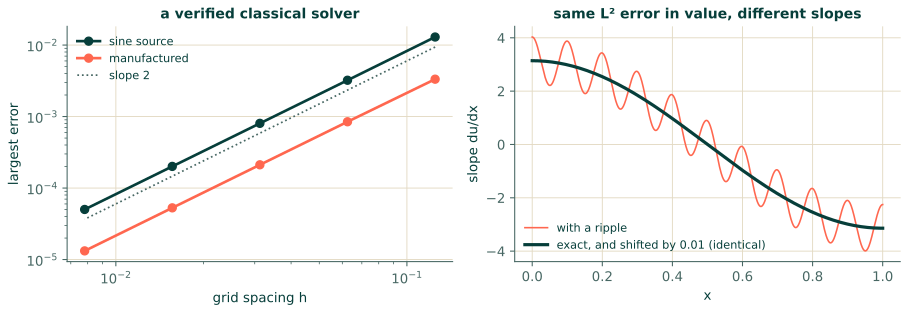
Each halving of the spacing $h$ divides the error by four: the observed order of convergence, $\log_2(e_h/e_{h/2})$, is 2, as the theory of the method predicts (Figure 4.4, left). That number is the point. A solver whose error falls at the predicted rate, on a problem with a known answer, has earned trust; it can then be run on a fine grid to serve as a reference where no formula exists. The finite-element column in Section 13.2 is the same idea in two dimensions.
A PINN has no $h$. Its error is set by the network, the points and the training, and it does not fall in a predictable way as you add points. That is why a PINN is compared against such solvers rather than verified in the same manner.
Measuring the gap
The usual single number is the relative $L^2$ error over a set of evaluation points,
$$\varepsilon_{L^2} = \frac{\lVert u_\theta - u_\text{ref}\rVert_2}{\lVert u_\text{ref}\rVert_2} = \sqrt{\frac{\sum_i \bigl(u_\theta(x_i) - u_\text{ref}(x_i)\bigr)^2}{\sum_i u_\text{ref}(x_i)^2}},$$
together with the largest pointwise error, $\max_i |u_\theta(x_i) - u_\text{ref}(x_i)|$. Neither says anything about derivatives, which is often what the engineer wants: stresses are derivatives of displacements, fluxes are derivatives of temperatures. Two approximations of $\sin(\pi x)$ with the same relative $L^2$ error show the difference:
xs = np.linspace(0, 1, 20001)
u, du = np.sin(np.pi * xs), np.pi * np.cos(np.pi * xs)
d, eps = 0.01, np.sqrt(2) * 0.01
candidates = {
    "shifted by 0.01 ": (u + d, du),
    "with a ripple   ": (u + eps * np.sin(20 * np.pi * xs), du + eps * 20 * np.pi * np.cos(20 * np.pi * xs)),
}
rel = lambda e, r: np.sqrt(np.mean(e**2)) / np.sqrt(np.mean(r**2))
for name, (v, dv) in candidates.items():
    print(f"{name} relative L2 {rel(v - u, u):.4f}   largest {np.abs(v - u).max():.4f}"
          f"   relative L2 of the slope {rel(dv - du, du):.3f}")
shifted by 0.01  relative L2 0.0141   largest 0.0100   relative L2 of the slope 0.000
with a ripple    relative L2 0.0141   largest 0.0141   relative L2 of the slope 0.283
By the usual measure the two are equally good. The first has a perfect slope; the second, whose small ripple is invisible in a plot of the values, gets the slope wrong by 28%. Section 2.4 warned that approximating a function well does not mean approximating its derivatives well. When derivatives matter, measure them.
A checklist for a reference
| Reference | Gives you | Costs you |
|---|---|---|
| Exact solution | the true answer, anywhere | exists only for simple linear problems |
| Manufactured solution | a known answer for any equation and domain | an invented problem, not the one you care about |
| Classical solver | an answer for the real problem | a mesh, a convergence study, and its own error |
Whatever the reference, evaluate on points the PINN did not train on, many more of them than it trained on, and report the error measure that matches what you will use the answer for.
Exercises
- A solver gives errors $4.0\times10^{-3}$ and $1.1\times10^{-3}$ on grids with $h = 0.1$ and $h = 0.05$. What is the observed order? Is it consistent with a second-order method?
- Manufacture a problem for $-u'' = f$ on $(0, 1)$ with the answer $u^\ast = \sin(3\pi x/2)$. What are $f$ and the end values? Which kind of condition fits the right end most naturally?
- A PINN for a beam returns a deflection with a relative $L^2$ error of $10^{-3}$. Why is that not enough to trust its bending stresses, which depend on $w''$?
Answers
- $\log_2(4.0/1.1) \approx 1.86$. Close to 2: on coarse grids the asymptotic rate is often not yet reached, so a second grid refinement would settle it.
- $f = -u^{\ast\prime\prime} = (3\pi/2)^2\sin(3\pi x/2)$. The end values are $u(0) = 0$ and $u(1) = \sin(3\pi/2) = -1$. The slope at $x = 1$ is $u^{\ast\prime}(1) = (3\pi/2)\cos(3\pi/2) = 0$, so an insulated (Neumann) right end, $u'(1) = 0$, also fits it exactly.
- The $L^2$ error of the deflection does not bound the error in its second derivative: a small, fast wiggle can leave $w$ almost unchanged and $w''$ badly wrong, as the ripple above did to the first derivative. Measure the error in $w''$ against a reference directly.
Recap
- Three references: exact solutions (best, rare), manufactured solutions (any equation, invented problem), classical solvers (the real problem, with their own verified error).
- A classical solver earns trust by converging at its predicted order on a problem with a known answer.
- Report relative $L^2$ and largest errors on fresh points, and measure derivative errors when derivatives are what you need.
References
- LeVeque, R. J. (2007). Finite difference methods for ordinary and partial differential equations: Steady-state and time-dependent problems. Society for Industrial and Applied Mathematics. doi:10.1137/1.9780898717839
- Roache, P. J. (2002). Code verification by the method of manufactured solutions. Journal of Fluids Engineering, 124(1), 4–10. doi:10.1115/1.1436090