Scientific ML Studio

A soft constraint (Section 6.3) is a request: the optimiser trades it against everything else in the loss, and a condition is only ever met approximately. There is an older idea, due to Lagaris et al. (1998), which predates the name PINN: write the trial function so that the conditions hold for every value of the weights. Then they are met exactly, and the loss contains the equation alone.

The construction

For Dirichlet conditions $u = g$ on the boundary, look for

$$u_\theta(\mathbf{x}) = G(\mathbf{x}) + D(\mathbf{x})\,N_\theta(\mathbf{x}),$$

where $N_\theta$ is the network, $G$ is any smooth function equal to $g$ on the boundary, and $D$ is a smooth function that is zero on the boundary and non-zero inside. On the boundary $D = 0$, so $u_\theta = G = g$ whatever the network outputs. Inside, the network supplies everything else. Some common cases:

Conditions	Trial function
$u(0) = a$, $u(1) = b$ on $[0, 1]$	$u = a(1 - x) + bx + x(1 - x)\,N(x)$
$u(x, 0) = u_0(x)$ (one initial condition)	$u = u_0(x) + t\,N(x, t)$
$u(0) = u_0$ and $u'(0) = v_0$ (two initial conditions)	$u = u_0 + v_0 t + t^2 N(t)$
$u = 0$ on the unit circle	$u = (1 - x^2 - y^2)\,N(x, y)$

For other shapes, $D$ can be built from distance functions, which are zero on each piece of the boundary and can be combined for complicated geometries; Sukumar & Srivastava (2022) work this out systematically, including how to treat Neumann and Robin conditions, which are harder because they constrain derivatives.

Poisson in one dimension, soft against hard

The problem of Section 6.1, $u'' = -\pi^2\sin(\pi x)$ with $u(0) = u(1) = 0$, trained three times each way with the same network, points and optimiser:

import math
import torch
import torch.nn as nn

def d(y, x):
    return torch.autograd.grad(y, x, torch.ones_like(y), create_graph=True)[0]

f = lambda x: -math.pi**2 * torch.sin(math.pi * x)
x_test = torch.linspace(0, 1, 1001).reshape(-1, 1)
exact = torch.sin(math.pi * x_test)

def train_poisson(hard, seed=0, epochs=3000):
    torch.manual_seed(seed)
    net = nn.Sequential(nn.Linear(1, 32), nn.Tanh(), nn.Linear(32, 32), nn.Tanh(),
                        nn.Linear(32, 32), nn.Tanh(), nn.Linear(32, 1))
    if hard:
        u = lambda x: x * (1 - x) * net(2 * x - 1)          # zero at both ends, whatever the weights
    else:
        u = lambda x: net(2 * x - 1)
    x_col = torch.rand(200, 1).requires_grad_(True)
    x_b = torch.tensor([[0.0], [1.0]])
    opt = torch.optim.Adam(net.parameters(), lr=1e-3)
    for epoch in range(epochs):
        opt.zero_grad()
        loss = ((d(d(u(x_col), x_col), x_col) - f(x_col)) ** 2).mean()
        if not hard:
            loss = loss + (u(x_b) ** 2).sum()                 # the boundary term only the soft version needs
        loss.backward()
        opt.step()
    with torch.no_grad():
        return ((u(x_test) - exact).norm() / exact.norm()).item(), u(x_b).abs().max().item()

for hard in (False, True):
    runs = [train_poisson(hard, seed) for seed in range(3)]
    print(f"{'hard' if hard else 'soft'}:  relative L2 errors " + "  ".join(f"{e:.1e}" for e, _ in runs)
          + f"    largest |u| at the ends {max(b for _, b in runs):.1e}")

soft:  relative L2 errors 4.8e-05  2.0e-04  7.5e-05    largest |u| at the ends 6.8e-05
hard:  relative L2 errors 1.7e-05  8.4e-05  5.6e-05    largest |u| at the ends 0.0e+00

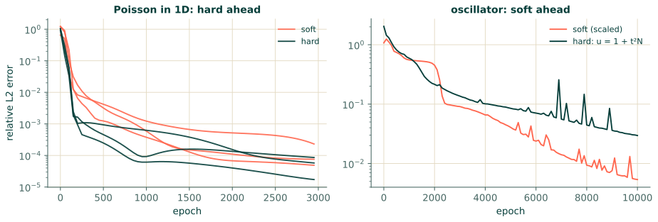
The hard version meets the boundary exactly, as it must, and in this experiment its error is also lower in each pair of runs. The network now has one job instead of two, and no weight decides how much the boundary matters against the equation.

What changes for the network

The construction does not come free. The network no longer represents $u$; it represents $N = (u - G)/D$, and that function can be harder. For Poisson above, $N = \sin(\pi x)/\bigl(x(1 - x)\bigr)$, a gentle curve between 3.14 and 4: easy. For the oscillator of Section 6.2, with $u = 1 + t^2 N(t)$, the network must learn $N = (u - 1)/t^2$, which near $t = 0$ is about $u''(0)/2 = -\omega^2/2 \approx -20$ and swings widely afterwards: a function far from the order-one outputs a freshly initialised network produces.

The effect can be measured. Hard initial conditions do remove the trivial solution that defeated the unscaled problem of Section 6.2: it is no longer available, since $u(0) = 1$ by construction. But on the scaled problem, which the soft version solved well, the hard version is worse:

zeta, omega, T = 0.1, 2 * math.pi, 2.0
omega_d = omega * math.sqrt(1 - zeta**2)
u_exact = lambda t: torch.exp(-zeta * omega * t) * (torch.cos(omega_d * t) + zeta * omega / omega_d * torch.sin(omega_d * t))
t_test = torch.linspace(0, T, 1001).reshape(-1, 1)

def train_oscillator_hard(epochs, seed=0, scaled=True):
    torch.manual_seed(seed)
    net = nn.Sequential(nn.Linear(1, 32), nn.Tanh(), nn.Linear(32, 32), nn.Tanh(),
                        nn.Linear(32, 32), nn.Tanh(), nn.Linear(32, 1))
    u = lambda t: 1 + t**2 * net(2 * t / T - 1)               # u(0) = 1 and u'(0) = 0 by construction
    t_col = (T * torch.rand(200, 1)).requires_grad_(True)
    opt = torch.optim.Adam(net.parameters(), lr=1e-3)
    for epoch in range(epochs):
        opt.zero_grad()
        u_c = u(t_col); u_t = d(u_c, t_col); u_tt = d(u_t, t_col)
        r = u_tt + 2 * zeta * omega * u_t + omega**2 * u_c
        if scaled:
            r = r / omega**2
        (r ** 2).mean().backward()
        opt.step()
    with torch.no_grad():
        return ((u(t_test) - u_exact(t_test)).norm() / u_exact(t_test).norm()).item()

print(f"hard, unscaled,  5000 epochs: error {train_oscillator_hard(5000, scaled=False):.1e}   (soft, unscaled: 0.98)")
print(f"hard, scaled,    5000 epochs: error {train_oscillator_hard(5000):.1e}")
print(f"hard, scaled,   10000 epochs: error {train_oscillator_hard(10000):.1e}   (soft, scaled: 5.5e-03)")

hard, unscaled,  5000 epochs: error 8.5e-02   (soft, unscaled: 0.98)
hard, scaled,    5000 epochs: error 8.5e-02
hard, scaled,   10000 epochs: error 3.0e-02   (soft, scaled: 5.5e-03)

Three observations. With hard initial conditions the unscaled problem no longer collapses to zero: the error is several per cent rather than 98%. Scaling the residual makes no difference to the hard version: with a single term in the loss, multiplying it by a constant leaves Adam's steps essentially unchanged (Section 3.5), so the first two runs coincide. And with the same network and the same 10000 epochs, the hard version ends several times worse than the soft, scaled one, because of the function it must represent. Figure 6.4 shows both comparisons over the course of training.

Left: relative error against epoch for the one-dimensional Poisson problem, three soft runs and three hard runs, the hard runs ending lower. Right: the same for the scaled oscillator, one soft run and one hard run, the soft run ending lower. — **Figure 6.4.** Soft and hard constraints, error against epoch. Left: Poisson in one dimension, three seeds each; the hard version is ahead. Right: the scaled oscillator; the hard version, $u = 1 + t^2N$, is behind, because $N$ must reach about $-20$ near $t = 0$.

When to build conditions in

Build a condition in when it is a simple Dirichlet or initial value on a simple shape, when the boundary must hold exactly (a fixed support, a symmetry), or when a soft version keeps converging to the wrong member of the family. Choose $D$ so that $N$ stays of order one: dividing by a factor that is tiny over much of the domain makes $N$ large there. And measure: the gain is not guaranteed.

Editing a Studio script

The Studio imposes every condition softly, as loss terms. Its generated script is plain Python, though, and the whole trial function passes through one helper, field, so a hard constraint is a few lines added after the module is loaded. For the 1D Poisson example, whose script ships with the book:

# not run
import poisson_1d as p                          # the generated script, saved as poisson_1d.py

soft_field = p.field
p.field = lambda pts, component=0: pts[:, 0:1] * (1 - pts[:, 0:1]) * soft_field(pts, component)
p.TERM_SCALES.update(bc1=0.0, bc2=0.0)          # the boundary terms are now zero by construction
history = p.train()

Every residual function in the script looks up field when it runs, so all of them now see the constrained trial function. On that script's settings (four layers of 40, 2000 points, 2000 epochs, three seeds) the patched version met the boundary exactly but did not beat the soft one: relative errors of $0.9$ to $1.7\times10^{-4}$, against $2.7$ to $6.1\times10^{-5}$ for the unpatched script. The script that produces these numbers is tools/figures_part3.py, function report_studio_patch. One problem, two network set-ups, opposite verdicts: which is why the box above ends as it does.

Exercises

Write a trial function on $[0, 1]$ that satisfies $u(0) = 2$ and $u(1) = -1$ for any network output.
For the heat equation on $0 < x < 1$ with $u(0, t) = u(1, t) = 0$ and $u(x, 0) = \sin(\pi x)$, write one trial function that satisfies all three conditions exactly.
Why is a Neumann condition, $u'(1) = h$, harder to build in than a Dirichlet one? Suggest a trial function for $u(0) = 0$, $u'(1) = 0$ on $[0, 1]$.

Answers

$u = 2(1 - x) - x + x(1 - x)\,N(x) = 2 - 3x + x(1 - x)\,N(x)$.
$u = \sin(\pi x) + t\,x(1 - x)\,N(x, t)$. At $t = 0$ the second term vanishes; at $x = 0$ and $x = 1$ both terms vanish.
A Neumann condition constrains the derivative of the trial function, which involves the network's derivative as well as its value, so a factor that merely vanishes on the boundary does not enforce it. Use factors whose slope vanishes there instead: $u = c\,x(2 - x) + x(1 - x)^2\,N(x)$, with $c$ a trainable number. Then $u(0) = 0$, and $u'(1) = c(2 - 2) + 0 = 0$ for every $N$ and $c$, because $(1 - x)^2$ and its derivative both vanish at $x = 1$. Distance-function methods (Sukumar & Srivastava, 2022) do this kind of construction systematically.

Recap

A trial function $u = G + D\,N$ satisfies Dirichlet and initial conditions exactly, for every value of the weights, and removes those terms and their weights from the loss.
The network must then represent $N = (u - G)/D$, which can be easy (Poisson here) or hard (the oscillator here).
Hard constraints rule out some failure modes, such as the trivial solution, but are not automatically more accurate. Measure, on your problem and your network.

Conditions built into the network

References

- Lagaris, I. E., Likas, A., & Fotiadis, D. I. (1998). Artificial neural networks for solving ordinary and partial differential equations. IEEE Transactions on Neural Networks, 9(5), 987–1000. doi:10.1109/72.712178
- Sukumar, N., & Srivastava, A. (2022). Exact imposition of boundary conditions with distance functions in physics-informed deep neural networks. Computer Methods in Applied Mechanics and Engineering, 389, 114333. doi:10.1016/j.cma.2021.114333