A first PINN, line by line

This section trains a complete PINN, from an empty file to an answer checked against an exact solution, and explains every line. The problem is an ordinary differential equation, so that nothing distracts from the method: one input, time, and one output.

The problem

A mass on a spring with some friction, pulled to one side and released. Its displacement $u(t)$ obeys

$$u'' + 2\zeta\omega\,u' + \omega^2 u = 0, \qquad u(0) = 1, \qquad u'(0) = 0,$$

with natural frequency $\omega = 2\pi$ (one oscillation per second) and damping ratio $\zeta = 0.1$, for $0 \le t \le 2$. Two initial conditions, because the equation is second order in time (Section 4.2): where the mass starts and how fast. The exact solution is a decaying cosine,

$$u(t) = e^{-\zeta\omega t}\left(\cos\omega_d t + \frac{\zeta\omega}{\omega_d}\sin\omega_d t\right), \qquad \omega_d = \omega\sqrt{1 - \zeta^2},$$

which the network never sees. We keep it to grade the answer.

The program

import math
import torch
import torch.nn as nn

zeta, omega, T = 0.1, 2 * math.pi, 2.0          # damping ratio, natural frequency (rad/s), time span (s)

def d(y, t):
    """dy/dt at every point, kept differentiable (Section 5.4)."""
    return torch.autograd.grad(y, t, torch.ones_like(y), create_graph=True)[0]

def train(scaled, epochs, seed=0):
    torch.manual_seed(seed)
    net = nn.Sequential(nn.Linear(1, 32), nn.Tanh(), nn.Linear(32, 32), nn.Tanh(),
                        nn.Linear(32, 32), nn.Tanh(), nn.Linear(32, 1))
    u = lambda t: net(2 * t / T - 1)                        # the trial function; inputs scaled to [-1, 1]
    t_col = (T * torch.rand(200, 1)).requires_grad_(True)   # collocation points in (0, T)
    t_0 = torch.zeros(1, 1, requires_grad=True)             # the start, where both conditions live
    opt = torch.optim.Adam(net.parameters(), lr=1e-3)
    history = []
    for epoch in range(epochs + 1):
        opt.zero_grad()
        u_c = u(t_col)
        u_t = d(u_c, t_col)
        u_tt = d(u_t, t_col)
        r = u_tt + 2 * zeta * omega * u_t + omega**2 * u_c       # the equation's residual
        u0 = u(t_0)
        v0 = d(u0, t_0)                                          # the initial velocity
        if scaled:                                               # measure time in units of 1/omega
            r, v0 = r / omega**2, v0 / omega
        loss_eq = (r ** 2).mean()
        loss_ic = ((u0 - 1) ** 2 + v0 ** 2).sum()
        loss = loss_eq + loss_ic
        loss.backward()
        opt.step()
        history.append((loss_eq.item(), loss_ic.item()))
    return u, history

omega_d = omega * math.sqrt(1 - zeta**2)
exact = lambda t: torch.exp(-zeta * omega * t) * (torch.cos(omega_d * t) + zeta * omega / omega_d * torch.sin(omega_d * t))
t_test = torch.linspace(0, T, 1001).reshape(-1, 1)          # 1001 points the network never trained on

Line by line:

• The network is the multilayer perceptron of Chapter 2: one input, three hidden layers of 32 tanh neurons, one output. tanh because the residual needs a second derivative (Section 5.4).
• u = lambda t: net(2 * t / T - 1) is the trial function. Time is scaled to $[-1, 1]$ inside the function, so autograd includes the factor $2/T$ in every derivative (Section 5.3).
• t_col holds 200 collocation points, drawn once, uniformly in $(0, T)$, with requires_grad=True so the network can be differentiated with respect to them.
• t_0 is the single point $t = 0$. Both initial conditions are imposed there: the value $u(0) = 1$, and the velocity $u'(0) = 0$, which is itself a derivative of the network.
• The residual is the equation with everything moved to one side, computed at all 200 points at once.
• The loss is the mean square of the residual plus the squares of the two initial-condition errors, with weights of 1 (Section 6.1). Then the four lines of every training loop (Section 3.6).

The scaled switch does nothing yet. It is there because of what happens next.

First attempt: a confident wrong answer

u_raw, hist_raw = train(scaled=False, epochs=5000)
with torch.no_grad():
    err = (u_raw(t_test) - exact(t_test)).norm() / exact(t_test).norm()
for e in (0, 1000, 5000):
    print(f"epoch {e:5d}:  equation loss {hist_raw[e][0]:.2e}   initial-condition loss {hist_raw[e][1]:.2e}")
print(f"relative L2 error against the exact solution: {err:.2f}")

epoch     0:  equation loss 4.41e+01   initial-condition loss 1.28e+00
epoch  1000:  equation loss 6.23e-03   initial-condition loss 9.86e-01
epoch  5000:  equation loss 1.54e-02   initial-condition loss 9.52e-01
relative L2 error against the exact solution: 0.98

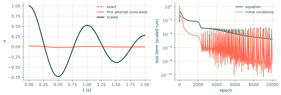
The equation loss fell from about 44 to about $10^{-2}$, which looks like training working. The initial-condition loss stayed near 1, and the answer is 98% wrong. Figure 6.2 shows why: the network has settled on a function close to $u = 0$. That is a perfectly good solution of the equation, which is homogeneous, and it violates only the initial value. The optimiser found that the cheapest way to reduce the total was to give up on one condition, which costs at most 1, and make the residual small, which at the start cost 44.

This is the most common way a PINN fails, and it has a name: convergence to a trivial solution. The loss does not warn you, because the loss is doing exactly what it was told. Only the comparison with a reference does.

Why, and the fix

Look at the sizes of the terms in the residual. For the true solution $u \sim 1$, the term $\omega^2 u$ is about $(2\pi)^2 \approx 39$, and $u''$ is of the same size with the opposite sign. So a modest relative mistake in the equation costs tens or hundreds in the loss, while abandoning the initial condition altogether costs 1. The imbalance is built in by the units, exactly as for the steel rod of Section 4.5.

The fix from Section 4.5 is to measure time in its natural unit, here $1/\omega$. With $\tau = \omega t$ the equation becomes $u_{\tau\tau} + 2\zeta u_\tau + u = 0$, every coefficient of order one, and $u_\tau(0) = u'(0)/\omega$. In the code that is exactly the scaled branch: divide the residual by $\omega^2$ and the velocity by $\omega$. Nothing else changes.

u_s, hist_s = train(scaled=True, epochs=10000)
with torch.no_grad():
    err = (u_s(t_test) - exact(t_test)).norm() / exact(t_test).norm()
for e in (0, 1000, 5000, 10000):
    print(f"epoch {e:5d}:  equation loss {hist_s[e][0]:.2e}   initial-condition loss {hist_s[e][1]:.2e}")
print(f"relative L2 error against the exact solution: {err:.1e}")

epoch     0:  equation loss 2.83e-02   initial-condition loss 1.28e+00
epoch  1000:  equation loss 8.82e-03   initial-condition loss 1.21e-04
epoch  5000:  equation loss 2.03e-04   initial-condition loss 7.63e-07
epoch 10000:  equation loss 1.66e-05   initial-condition loss 1.04e-07
relative L2 error against the exact solution: 5.5e-03

The initial-condition loss now falls first and fastest, the equation follows, and the answer is within a fraction of a per cent of the exact solution over two full oscillations.

What to take from it

Three points, each of which returns throughout the book.

1. A falling loss is not a correct answer. The first attempt's loss fell by a factor of three thousand on the equation term. Check against a reference (Section 4.4), and look at every term of the loss, not only the total.
2. Scale before you train. The same network, points and optimiser went from 98% wrong to under 1% wrong because the equation was written in its natural units. Chapter 10 treats the weights of the loss as a design decision in their own right; scaling is the first and cheapest part of it.
3. The result depends on the run. Change the seed in train and the scaled error moves: with seed=1 it is about twice as large, with seed=2 somewhat smaller. Section 6.5 explains what to report.

Exercises

1. Change $\zeta$ to 0 (no friction). What is the exact solution? Does the scaled PINN still find it over $[0, 2]$?
2. Set T = 4.0 (four oscillations) with the scaled loss. Predict, then check: is the error larger or smaller?
3. Instead of scaling, give the initial-condition term a weight of 100 in the unscaled loss. Why should that also help, and why is scaling still the better habit?

Recap

• A PINN is the training loop of Chapter 3 with a loss made of residuals: the equation at collocation points and each condition at its points, all derivatives by autograd.
• An unscaled oscillator converged to the trivial solution $u \approx 0$: the loss fell, the answer was wrong.
• Writing the equation in natural units balanced the terms and gave a sub-per-cent error. Check every answer against a reference, and every loss term on its own.