Scientific ML Studio

The equation $x^2 = 2$ asks for a number, and $x = \sqrt2$ answers it. A differential equation asks for a function. It does not say what the function is. It says how the function changes, and leaves you to find the functions that change that way.

Part 1 gave us a model that can represent almost any function, and a way to adjust it. This part of the book is about the other half of a PINN: the equations it is asked to satisfy. This section fixes the vocabulary.

The smallest example

A cup of coffee cools at a rate proportional to how much hotter it is than the room. Write $T(t)$ for its temperature above room temperature, in kelvin, at time $t$. Newton's law of cooling says

$$\frac{dT}{dt} = -k\,T,$$

where $k > 0$ is a constant that depends on the cup. Any function whose slope is $-k$ times its own value will do, and there are many. SymPy can find them all:

import sympy as sp

t, k = sp.symbols("t k", positive=True)
T = sp.Function("T")

general = sp.dsolve(sp.Eq(T(t).diff(t), -k * T(t)))
print("general solution :", general)

particular = sp.dsolve(sp.Eq(T(t).diff(t), -k * T(t)), ics={T(0): 60})
print("with T(0) = 60   :", particular)

general solution : Eq(T(t), C1*exp(-k*t))
with T(0) = 60   : Eq(T(t), 60*exp(-k*t))

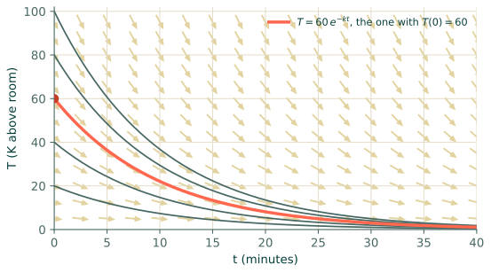
The equation alone gives a family of solutions, $T(t) = C_1 e^{-kt}$, one for every value of the constant $C_1$. Figure 4.1 draws a few. To pick one you need one more fact, here the temperature at the start: a cup that is 60 K above the room at $t = 0$ follows $T = 60\,e^{-kt}$ and no other curve. That extra fact is an initial condition, and the next section is about such conditions.

Short arrows showing the slope prescribed by dT/dt = -kT at many points of the (t, T) plane, with five exponential decay curves following the arrows; the one that starts at T = 60 is drawn thicker and marked with a dot at t = 0. — **Figure 4.1.** The equation $dT/dt = -kT$ (here $k = 0.1$ per minute) prescribes a slope at every point, drawn as short arrows. Every curve that follows the arrows is a solution. The initial condition $T(0) = 60$ picks one of them.

The vocabulary

A handful of words describe any differential equation, and they decide which methods apply.

The unknown is the function we are after: $T$ above, or $u$ in most of this book.
The independent variables are its inputs: time $t$, and position $x$ (or $x, y$).
An ordinary differential equation (ODE) has one independent variable. A partial differential equation (PDE) has several, and its derivatives are partial derivatives, such as $\partial u/\partial t$.
The order is the highest derivative that appears. Newton's law of cooling is first order. The heat equation $u_t = a\,u_{xx}$ is first order in time and second order in space.
An equation is linear if the unknown and its derivatives appear only to the first power, multiplied by known coefficients. Otherwise it is nonlinear.
A term that does not involve the unknown at all, such as a heat source, is a source term or forcing. Without one the equation is homogeneous.

We write partial derivatives with subscripts, so $u_t = \partial u/\partial t$ and $u_{xx} = \partial^2 u/\partial x^2$, and $\nabla^2 u = u_{xx} + u_{yy}$ is the Laplacian.

Linear means superposition

Linearity has a practical meaning. Write the equation as an operator $\mathcal{N}$ acting on the unknown, $\mathcal{N}[u] = f$. For the heat equation, $\mathcal{N}[u] = u_t - a\,u_{xx}$. The operator is linear when $\mathcal{N}[u + v] = \mathcal{N}[u] + \mathcal{N}[v]$ (and constants factor out), which means that solutions can be added: two solutions of the homogeneous equation add up to a third. The check is mechanical, so let SymPy do it for the heat operator and for Burgers' operator $u_t + u\,u_x - \nu\,u_{xx}$:

x, a, nu = sp.symbols("x a nu", positive=True)
u, v = sp.Function("u")(x, t), sp.Function("v")(x, t)

heat = lambda w: sp.diff(w, t) - a * sp.diff(w, x, 2)
burgers = lambda w: sp.diff(w, t) + w * sp.diff(w, x) - nu * sp.diff(w, x, 2)

for name, N in [("heat", heat), ("Burgers", burgers)]:
    gap = sp.expand(N(u + v) - N(u) - N(v))
    print(f"{name:8s} N[u + v] - N[u] - N[v] = {gap}")

heat     N[u + v] - N[u] - N[v] = 0
Burgers  N[u + v] - N[u] - N[v] = u(x, t)*Derivative(v(x, t), x) + v(x, t)*Derivative(u(x, t), x)

The heat operator passes. Burgers' leaves behind $u\,v_x + v\,u_x$, the cross terms of the product $u\,u_x$, so it is nonlinear: two of its solutions do not add up to a third.

This matters for what follows. For a linear equation there are exact formulas in many simple cases (built, as Section 4.4 shows, by adding up simple solutions), and the residual is a linear function of the network's output. For a nonlinear one there usually is no formula, and the residual of a PINN contains products of the network with its own derivatives, which makes the loss harder to minimise. Burgers' equation in Section 13.6 is the example.

The equations in this book

Equation	Written as	Order	Linear	Describes	Where
Decay	$T' = -kT$	1	yes	cooling, radioactive decay	this section
Damped oscillator	$u'' + 2\zeta\omega\,u' + \omega^2 u = 0$	2	yes	a mass on a spring, vibration	6.2
Heat, diffusion	$u_t = a\,u_{xx}$	1 in $t$, 2 in $x$	yes	conduction, diffusion	13.3
Wave	$u_{tt} = c^2 u_{xx}$	2	yes	strings, sound	13.5
Poisson, Laplace	$\nabla^2 u = f$	2	yes	steady heat, electrostatics, membranes	13.1, 13.2, 13.7
Advection	$u_t + c\,u_x = 0$	1	yes	something carried along at speed $c$	8.2
Burgers	$u_t + u\,u_x = \nu\,u_{xx}$	2	no	shocks, a one-dimensional model of fluid flow	13.6
Euler–Bernoulli beam	$EI\,w'''' = q$	4	yes	the bending of a beam under a load $q$	8.5

Every one of them comes from a conservation law (of energy, momentum or mass) plus a rule that closes it, such as Fourier's law for heat flux. The physical meaning will matter when we choose conditions and scales in the next sections.

Checking a solution

To check that a function solves an equation, substitute it and see whether the equation holds at every point. For the heat equation the functions $u = e^{-a n^2 \pi^2 t}\sin(n\pi x)$, one for each whole number $n$, are solutions:

n = sp.symbols("n", integer=True, positive=True)
u = sp.exp(-a * n**2 * sp.pi**2 * t) * sp.sin(n * sp.pi * x)

residual = sp.diff(u, t) - a * sp.diff(u, x, 2)
print("u_t - a u_xx =", sp.simplify(residual))

u_t - a u_xx = 0

The difference $u_t - a\,u_{xx}$ simplifies to zero for every $n$, $x$ and $t$. Written that way, with everything on one side, it has a name: the residual. It is zero for a solution and non-zero for anything else, and Section 1.2 already used it as a loss.

Where this goes in a PINN

The first step in setting up any PINN is to write the equation in residual form, $r = \mathcal{N}[u] - f$, so that the goal is "make $r$ zero everywhere". For the heat equation that is $r = u_t - a\,u_{xx}$. For Poisson's equation $-u'' = \pi^2\sin(\pi x)$, written the way the Studio writes it, it is $r = u'' - f$ with $f = -\pi^2\sin(\pi x)$. A PINN computes $r$ for its network at many points and pushes it towards zero (Raissi et al. (2019)). The conditions of the next section are residuals too.

Exercises

Give the order of each equation and say whether it is linear: (a) $u_t = u_{xx} + u^2$; (b) $u'' + \sin(x)\,u = 0$; (c) $u_t + u_{xxx} = 0$; (d) $u_x^2 + u_y^2 = 1$.
Show that $u = \sin(x - ct)$ solves the advection equation $u_t + c\,u_x = 0$. Does $u = g(x - ct)$ solve it for any differentiable function $g$?
Write the beam equation $EI\,w'''' = q$ in residual form. If $EI$ is constant and $q$ is a uniform load, what kind of function must $w$ be?

Answers

(a) Second order, nonlinear (the $u^2$ term). (b) Second order, linear: the coefficient $\sin x$ depends on $x$, not on $u$, which is allowed. (c) Third order, linear. (d) First order, nonlinear (the squares of the derivatives).
$u_t = -c\cos(x - ct)$ and $u_x = \cos(x - ct)$, so $u_t + c\,u_x = 0$. For any $g$, the chain rule gives $u_t = -c\,g'(x - ct)$ and $u_x = g'(x - ct)$, so yes: every profile that slides to the right at speed $c$ without changing shape is a solution.
$r = EI\,w'''' - q$. With $EI$ and $q$ constant, $w'''' = q/EI$ is a constant, so $w$ is a polynomial of degree four. Its four free coefficients are fixed by four conditions at the beam's ends.

Recap

A differential equation prescribes how a function changes; its solutions form a family, and extra conditions pick one.
Order, ODE or PDE, linear or nonlinear: these decide which methods apply. Linear equations allow superposition; nonlinear ones, such as Burgers', do not.
Written in residual form, $r = \mathcal{N}[u] - f$, an equation becomes a quantity that should be zero. That is what a PINN minimises.

What a differential equation says

References

- Raissi, M., Perdikaris, P., & Karniadakis, G. E. (2019). Physics-informed neural networks: A deep learning framework for solving forward and inverse problems involving nonlinear partial differential equations. Journal of Computational Physics, 378, 686–707. doi:10.1016/j.jcp.2018.10.045