Second and mixed derivatives

Section 5.3 produced first derivatives of a network with one call. The heat equation needs $u_{xx}$, Poisson's equation needs $u_{xx} + u_{yy}$, and the beam equation of Section 4.1 needs $w''''$. Each is a derivative of a derivative, and create_graph=True is what makes that possible: it keeps the first derivative attached to the record, so that it can be differentiated in its turn. This section builds the higher derivatives, checks them, shows the activation failure promised in Section 2.3, and measures what they cost.

A helper, and a check against a known function

Every residual in the rest of the book uses one small helper: the derivative of a column y with respect to the points, kept differentiable.

import math
import time
import torch
import torch.nn as nn

def d(y, pts):
    """dy/dpts at every point, one column per coordinate, still differentiable."""
    return torch.autograd.grad(y, pts, torch.ones_like(y), create_graph=True)[0]

A second derivative is d applied to one column of a first derivative. For $u = \sin(\pi x)\sin(\pi y)$ the Laplacian should be $-2\pi^2 u$ exactly:

pts = torch.rand(1000, 2, dtype=torch.float64, requires_grad=True)
x, y = pts[:, 0:1], pts[:, 1:2]
u = torch.sin(math.pi * x) * torch.sin(math.pi * y)

g = d(u, pts)                       # columns u_x, u_y
u_xx = d(g[:, 0:1], pts)[:, 0:1]    # differentiate u_x, keep the x column
u_yy = d(g[:, 1:2], pts)[:, 1:2]    # differentiate u_y, keep the y column
print("largest |u_xx + u_yy + 2 pi^2 u|:", f"{(u_xx + u_yy + 2 * math.pi**2 * u).abs().max().item():.1e}")

largest |u_xx + u_yy + 2 pi^2 u|: 3.6e-15

Rounding error only. The pattern generalises: one call for the gradient, then one call per second derivative you need. A Laplacian in $d$ dimensions takes $1 + d$ calls, because each $u_{x_ix_i}$ comes from a separate column.

Mixed derivatives

Differentiating the $x$ column with respect to $y$ gives $u_{xy}$; differentiating the $y$ column with respect to $x$ gives $u_{yx}$. For a smooth function they are equal, and for a tanh network they are, to rounding:

torch.manual_seed(0)
net = nn.Sequential(nn.Linear(2, 32), nn.Tanh(), nn.Linear(32, 32), nn.Tanh(), nn.Linear(32, 1)).double()
p = torch.rand(1000, 2, dtype=torch.float64, requires_grad=True)

g = d(net(p), p)
u_xy = d(g[:, 0:1], p)[:, 1:2]
u_yx = d(g[:, 1:2], p)[:, 0:1]
print("largest |u_xy - u_yx|:", f"{(u_xy - u_yx).abs().max().item():.1e}")

largest |u_xy - u_yx|: 3.5e-17

So one of the two calls is enough, which is why the Studio's custom residual accepts only u_xy, never u_yx (Choose the equation).

Why ReLU cannot be used

Section 2.3 argued that a ReLU network is piecewise linear, so its second derivative is zero almost everywhere, and promised to show it with automatic differentiation. Take the residual of $u'' = f$, with $f = -\pi^2\sin(\pi x)$, for a ReLU network and for a tanh network of the same shape, and compute the gradient of its mean square with respect to the weights, the quantity training would follow:

xs = torch.rand(200, 1, requires_grad=True)
f = (-math.pi**2 * torch.sin(math.pi * xs)).detach()       # the source does not depend on the network

for name, act in [("ReLU", nn.ReLU()), ("tanh", nn.Tanh())]:
    torch.manual_seed(0)
    m = nn.Sequential(nn.Linear(1, 32), act, nn.Linear(32, 32), act, nn.Linear(32, 1))
    u_xx = d(d(m(xs), xs), xs)
    loss = ((u_xx - f) ** 2).mean()
    m.zero_grad()
    loss.backward()
    grad_norm = torch.sqrt(sum((q.grad ** 2).sum() for q in m.parameters() if q.grad is not None))
    print(f"{name}: largest |u_xx| {u_xx.abs().max().item():.2e}   size of the gradient {grad_norm.item():.2e}")

ReLU: largest |u_xx| 0.00e+00   size of the gradient 0.00e+00
tanh: largest |u_xx| 1.48e-01   size of the gradient 1.40e+01

For the ReLU network $u_{xx}$ is exactly zero at every point, the residual is $-f$ whatever the weights are, and the gradient is zero: training cannot move. Automatic differentiation reports the derivative of each piece and has nothing to say about the kinks between pieces, where the true second derivative is an infinite spike. The tanh network has a curvature that depends on its weights, and a gradient to follow. Figure 5.4 shows the same contrast after both networks have been fitted to $\sin(2\pi x)$ by ordinary regression.

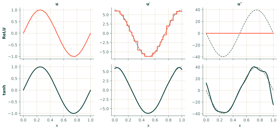
The figure carries a warning beyond PINNs: a network can fit values well and its derivatives badly, and a plot of the values will not tell you. Section 4.4 made the same point with a ripple.

What higher derivatives cost

Each extra derivative is a further sweep over a recorded computation that grows with every sweep. Here are the costs, relative to one forward pass, for a network of four layers of forty (the Studio's default) on 2000 points in two dimensions, with and without the backward pass that training adds on top:

torch.manual_seed(0)
layers = [nn.Linear(2, 40), nn.Tanh()]
for _ in range(3):
    layers += [nn.Linear(40, 40), nn.Tanh()]
net = nn.Sequential(*layers, nn.Linear(40, 1))
P = torch.rand(2000, 2, requires_grad=True)

def value():
    return net(P)
def gradient():
    return d(net(P), P)
def laplacian():
    g = d(net(P), P)
    return d(g[:, 0:1], P)[:, 0:1] + d(g[:, 1:2], P)[:, 1:2]
def and_train(fn):
    def run():
        net.zero_grad()
        (fn() ** 2).mean().backward()
    return run

def best_time(fn, reps=30):
    times = []
    for _ in range(reps):
        t0 = time.perf_counter(); fn(); times.append(time.perf_counter() - t0)
    return min(times)

base = best_time(value)
for name, fn in [("u", value), ("u_x and u_y", gradient), ("Laplacian", laplacian)]:
    print(f"{name:12s} {best_time(fn) / base:5.1f} x one forward pass,"
          f"  {best_time(and_train(fn)) / base:5.1f} x with the training backward pass")

u              1.2 x one forward pass,    4.4 x with the training backward pass
u_x and u_y    3.2 x one forward pass,   10.9 x with the training backward pass
Laplacian     16.2 x one forward pass,   34.8 x with the training backward pass

The exact ratios depend on the machine and vary from run to run; the pattern does not. The Laplacian of a two-input network costs more than ten forward passes, and the training step on top of it roughly doubles that. This is why a PINN epoch on 2000 points costs far more than an epoch of ordinary regression on 2000 points, and why fourth derivatives, as in the beam equation, are worth avoiding when an equation can be rewritten with lower ones. Section 8.5 does exactly that for a beam.

Exercises

1. How many calls to d does the Laplacian of $u(x, y, z)$ need? How many for all six distinct second derivatives?
2. A GELU activation is smooth but close to ReLU for large inputs. Would you expect it to have the same problem as ReLU? (Try it: replace nn.ReLU() by nn.GELU() above.)
3. The residual of the beam equation needs $w''''$. Starting from $w$, how many nested calls to d is that, and roughly how does its cost compare with $w''$ on the timing above?

Recap

• A second derivative is the derivative of one column of the first, which create_graph=True makes possible. A Laplacian in $d$ dimensions takes $1 + d$ calls; mixed derivatives come out symmetric.
• A ReLU network has zero second derivative and gives a residual loss with zero gradient. Use smooth activations whenever the equation has second or higher derivatives.
• Higher derivatives are expensive: more than ten forward passes for a two-dimensional Laplacian, about twice that with the training step, and more for each further order.