A simply supported beam: PINN against FEM
A simply supported beam: PINN against FEM
A beam rests on two supports and carries the same load along its whole length. How far does it bend, and what bending moment and shear force does it carry? This lesson answers both questions with a physics-informed neural network (PINN) built in the Studio. It then checks the answer in two independent ways: against the exact solution, and against a finite element (FEM) solution.
The beam is a good test because the answer is known exactly. It also asks more of the network than the deflection alone: the moment needs the network's second derivative, and the shear force needs its third.
1. The problem
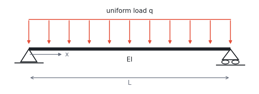
Figure 1. The simply supported beam. The left support is a pin, the right support is a roller, and the load $q$ (force per unit length) is the same everywhere.
We use the Euler-Bernoulli beam model. It assumes the beam is slender, the deflection is small, and cross-sections stay plane and perpendicular to the bent axis (no shear deformation). Under these assumptions the deflection $w(x)$, measured downward, obeys
$$ EI\,\frac{d^4 w}{dx^4} = q, \qquad 0 < x < L, $$
where $E$ is Young's modulus and $I$ the second moment of area of the cross-section. The product $EI$ is the bending stiffness, and here it is the same along the beam.
A fourth-order equation needs four conditions, two at each end. Neither support lets the beam move up or down, and neither resists rotation, so the bending moment there is zero:
$$ w(0) = w(L) = 0, \qquad w''(0) = w''(L) = 0 . $$
Once $w$ is known, three more quantities follow from its derivatives:
| Quantity | Formula | Derivative of $w$ |
|---|---|---|
| Slope (rotation of the cross-section) | $\theta = w'$ | first |
| Bending moment | $M = -EI\,w''$ | second |
| Shear force | $V = \dfrac{dM}{dx} = -EI\,w'''$ | third |
The exact solution is a standard result:
$$ w(x) = \frac{q\,x}{24\,EI}\left(L^3 - 2Lx^2 + x^3\right), \qquad w_{\max} = w\!\left(\tfrac{L}{2}\right) = \frac{5\,qL^4}{384\,EI}. $$
2. From four derivatives to two
The Studio cannot take this equation as written. A Custom residual can use derivatives up to the second order (u_xx), and a boundary condition can set only $u$ or its normal derivative, not $w''$ (see Choose the equation and Set the boundary and initial conditions).
This beam does not need the fourth-order form. It is statically determinate: the two support reactions, $qL/2$ each, follow from equilibrium alone, and so does the bending moment at every point:
$$ M(x) = \frac{q\,x\,(L - x)}{2}. $$
Put this into $M = -EI\,w''$ and the problem becomes second order:
$$ EI\,w'' = -\frac{q\,x\,(L-x)}{2}, \qquad w(0) = w(L) = 0 . $$
This is the classical double integration method of beam theory. Two conditions are enough now, because the moment conditions $M(0) = M(L) = 0$ are already built into $M(x)$.
This route works only when statics gives $M(x)$. A beam clamped at both ends, or clamped at one end and propped at the other, is statically indeterminate: its moment depends on the deflection, and it needs the fourth-order equation.
Scaling
We measure length in units of $L$ and deflection in units of its exact maximum $w_{\max}$:
$$ \hat{x} = \frac{x}{L}, \qquad u = \frac{w}{w_{\max}}. $$
The equation becomes (dropping the hat on $x$)
$$ u'' = -38.4\,x\,(1-x), \qquad u(0) = u(1) = 0, \qquad 0 < x < 1, $$
since $384/(5 \cdot 2) = 38.4$. Its exact solution is
$$ u(x) = 3.2\,x\,(1 - 2x^2 + x^3), $$
which is 0 at both ends and exactly 1 at the middle. Scaling the answer to a peak of 1 is not essential, but it puts the problem on the same footing as the 1D Poisson example, whose answer also peaks at 1, so the default network and loss weights suit it.
In these units the slope is $u'$, the moment is $-u''$ and the shear force is $-u'''$. To get back to physical values, multiply by $w_{\max}$, $w_{\max}/L$, $EI\,w_{\max}/L^2$ and $EI\,w_{\max}/L^3$ respectively. For example, the scaled shear at the left support is $38.4$, and $38.4 \times 5qL/384 = qL/2$, the support reaction.
3. Build it in the Studio
The build is the empty-canvas Poisson notebook with a different source and one extra tick.
- Start. Open the Studio. Name the notebook Simply supported beam, choose An empty canvas, and press Create notebook.
- Place ten blocks: Domain, PDE, Boundary condition (two of them), Network, Loss, Optimiser, Train, Visualisation and Report.
- Domain. Geometry type Line, x min
0, x max1, Time dimension off. Press Detect boundaries: it reports two boundaries, BC1 at $x = 0$ and BC2 at $x = 1$. - PDE. Equation type Elliptic, Equation Poisson. In Source f(x, y) type:
text
   -38.4*x*(1-x)
The Studio's Poisson block solves $\nabla^2 u = f$, which in 1D is $u'' = f$. So $f$ is the right-hand side exactly as written above, minus sign included.
5. BC 1 and BC 2. Condition type Dirichlet, u = 0.0. Each one fixes the deflection at one support.
6. Optimiser. Keep Adam, learning rate 0.001 and 5000 epochs, and tick Second stage (L-BFGS).
7. Network, Loss, Train, Visualisation, Report. Leave the defaults: four hidden layers of 40 neurons with tanh, equal loss weights, seed 0, a field plot, a loss curve and a results table.
8. Wire them. The same thirteen wires as in the Poisson notebook:
| # | From | To |
|---|---|---|
| 1 | Domain Coords | PDE Coords |
| 2 | Domain Interior | PDE Interior |
| 3 | Domain Coords | Network Coords |
| 4 | Domain BC1 | BC 1 Boundary |
| 5 | Domain BC2 | BC 2 Boundary |
| 6 | PDE PDE residual | Loss PDE residual |
| 7 | Network Network | Loss Network |
| 8 | BC 1 output | Loss BC / IC |
| 9 | BC 2 output | Loss BC / IC |
| 10 | Loss Loss | Train Loss |
| 11 | Optimiser Optimiser | Train Optimiser |
| 12 | Train Model | Visualisation Model |
| 13 | Train Model | Report Model |
- Check and generate. The Graph check should read nothing to flag. Press Generate code, then Download .py. Press Download notebook as well, to keep the canvas.
4. Run it
Put the script in an empty folder (or upload it to Colab and put ! before each command). Try a short run first, to catch a typing mistake in seconds:
python simply-supported-beam.py --epochs 200
Then train three times. Each run saves its weights to its own file:
python simply-supported-beam.py --checkpoint run1.pt --no-plots
python simply-supported-beam.py --checkpoint run2.pt --no-plots
python simply-supported-beam.py --checkpoint run3.pt
Why three? The script builds the network before it sets the random seed (see Read the script), so every run starts from different weights. Three runs show how much the answer depends on the start. Only the last run draws figures, so figures/ and results.csv both belong to run 3.
5. What came out
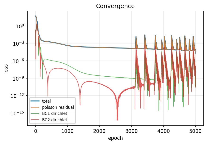
Figure 2. figures/loss.png from run 3. The total is almost entirely the residual of the equation. The boundary terms (green and red) are tiny: the network pins both ends down early.
Two features of the loss curve are worth knowing:
- The boundary terms are far smaller than the residual. The supports are easy to satisfy. The hard part is getting the curvature right everywhere in between.
- From about epoch 3000 the loss spikes repeatedly, jumping by two or three orders of magnitude and recovering each time. This is Adam overshooting near a minimum. It is the reason to tick the second stage: L-BFGS starts from wherever Adam stopped and settles into the minimum.
figures/field.png shows a single smooth hump from 0 to 1 and back. The Studio plots $u$ upward; the beam itself bends downward.
A quick check
results.csv holds the network's value at the 2000 interior training points. A few lines compare it with the exact solution:
import csv, math

xs, us = [], []
with open("results.csv") as f:
    for row in csv.reader(f):
        if not row or row[0].startswith("#") or row[0] == "x":
            continue                     # blank line, summary block, header
        xs.append(float(row[0]))
        us.append(float(row[1]))

exact = [3.2 * x * (1 - 2 * x**2 + x**3) for x in xs]
num = math.sqrt(sum((u - e) ** 2 for u, e in zip(us, exact)))
den = math.sqrt(sum(e ** 2 for e in exact))
print(f"{len(xs)} points, relative L2 error = {num / den:.2e}")
For run 3 this prints a relative L2 error of $8.1 \times 10^{-6}$.
If the error is near 2, the deflection came out upside down and the source was typed with the wrong sign. If it is around 0.1 or larger, check the source formula character by character.
6. A closer look: PINN, FEM and the exact answer
The check above uses the training points and the deflection only. The comparison script beam_compare.py goes further. Put it next to the Studio script and run
python beam_compare.py --script simply-supported-beam.py --checkpoint run1.pt run2.pt run3.pt --results results.csv
It loads each trained network and evaluates it on 2001 evenly spaced points. It also finds the network's first, second and third derivatives by automatic differentiation, the same tool the Studio uses to train it. That gives the PINN's slope, moment and shear. It then compares all four against the exact solution, and against a finite element solution.
The FEM reference. The finite element solution solves the full fourth-order equation $EI\,w'''' = q$, not the reduced one. It uses 16 equal Euler-Bernoulli beam elements. Each element has cubic Hermite shape functions, with the deflection and the slope as unknowns at each node. The supports set $w = 0$; $w'' = 0$ needs no constraint, because it is a natural condition of this formulation. The moment and shear come from differentiating the element shape functions. The code is plain NumPy and SciPy, inside the script.
The script also checked the generated code: the residual inside the script equals $u'' + 38.4\,x(1-x)$ to within $2 \times 10^{-7}$. So the Studio solved the equation we meant it to.
The deflection
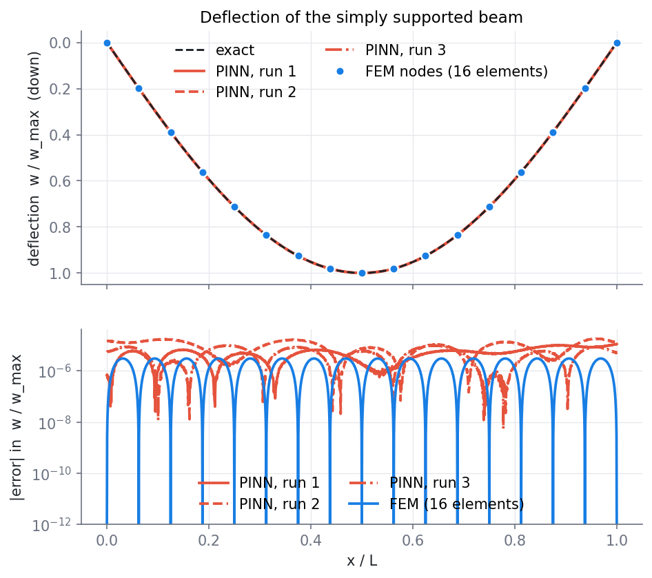
Figure 3. Deflection (scaled, drawn downward) and its error. Red: the three PINN runs. Blue: FEM with 16 elements. Dashed: exact.
On the scale of the beam, the network, the FEM and the exact solution cannot be told apart. The error plot separates them:
- FEM is exact at its nodes (to round-off, about $10^{-12}$). That is a known property of Hermite beam elements under this kind of load. Between the nodes its error rises to about $3 \times 10^{-6}$ of $w_{\max}$.
- The PINN has a smooth error spread over the whole beam, between about $10^{-6}$ and $2 \times 10^{-5}$ of $w_{\max}$. It is a little larger than the FEM error.
Slope, moment and shear
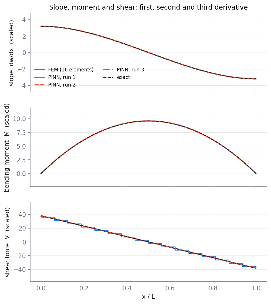
Figure 4. The slope, moment and shear force, from the first, second and third derivatives of each solution.
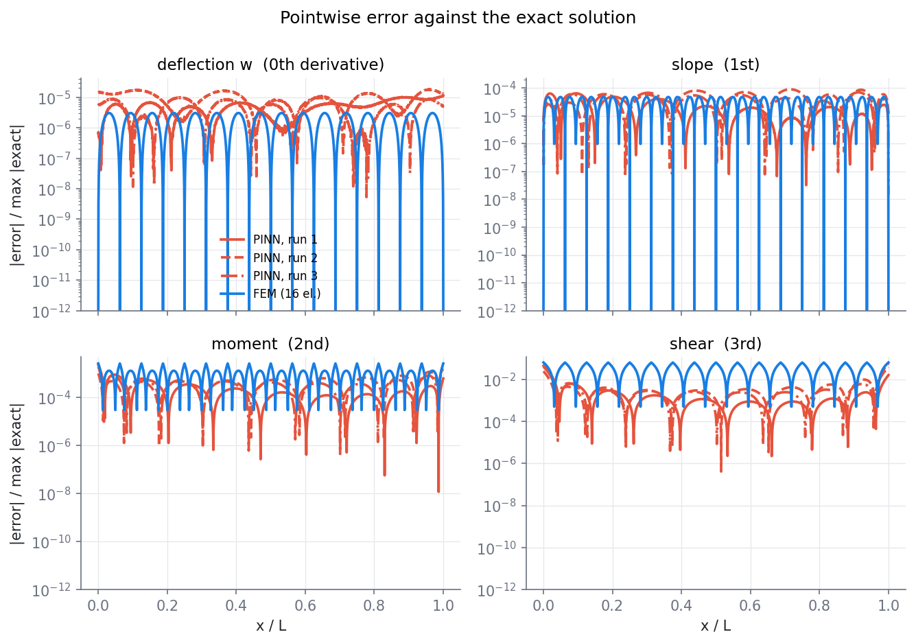
Figure 5. Pointwise error, divided by the largest exact value of each quantity, for the PINN runs (red) and FEM with 16 elements (blue).
The pattern in Figure 5 is the main lesson of this page: every derivative costs accuracy, for both methods.
- FEM. Within each element the deflection is a cubic polynomial. Its second derivative (the moment) is therefore a straight line on each element, and its third derivative (the shear) is a constant, a staircase over the beam. Each derivative loses one order of accuracy.
- PINN. The network is a smooth function, so its derivatives are smooth too, and they lose accuracy more slowly here. The weak points are the two ends. The residual is largest there, and so are the moment and shear errors.
The numbers
All errors are relative to the exact solution on the 2001-point grid. Relative L2 is the root-mean-square error divided by the root-mean-square exact value. Relative max is the largest error divided by the largest exact value.
| Quantity | Metric | PINN run 1 | PINN run 2 | PINN run 3 | FEM, 16 elements |
|---|---|---|---|---|---|
| Deflection $w$ | rel. L2 | $7.9 \times 10^{-6}$ | $1.5 \times 10^{-5}$ | $8.0 \times 10^{-6}$ | $2.7 \times 10^{-6}$ |
| rel. max | $1.1 \times 10^{-5}$ | $1.8 \times 10^{-5}$ | $1.0 \times 10^{-5}$ | $3.1 \times 10^{-6}$ | |
| Slope $\theta$ | rel. L2 | $3.7 \times 10^{-5}$ | $6.9 \times 10^{-5}$ | $5.6 \times 10^{-5}$ | $4.8 \times 10^{-5}$ |
| rel. max | $6.4 \times 10^{-5}$ | $8.9 \times 10^{-5}$ | $6.9 \times 10^{-5}$ | $4.7 \times 10^{-5}$ | |
| Moment $M$ | rel. L2 | $4.2 \times 10^{-4}$ | $6.6 \times 10^{-4}$ | $5.7 \times 10^{-4}$ | $1.6 \times 10^{-3}$ |
| rel. max | $2.3 \times 10^{-3}$ | $2.4 \times 10^{-3}$ | $1.9 \times 10^{-3}$ | $2.6 \times 10^{-3}$ | |
| Shear $V$ | rel. L2 | $8.9 \times 10^{-3}$ | $1.2 \times 10^{-2}$ | $1.1 \times 10^{-2}$ | $6.3 \times 10^{-2}$ |
| rel. max | $4.4 \times 10^{-2}$ | $5.6 \times 10^{-2}$ | $4.0 \times 10^{-2}$ | $6.3 \times 10^{-2}$ |
And at the points an engineer would read first (scaled units):
| Value | Exact | PINN run 1 | PINN run 2 | PINN run 3 |
|---|---|---|---|---|
| Mid-span deflection $u(0.5)$ | 1 | 1.000002 | 0.999993 | 0.999994 |
| Slope at the left support $u'(0)$ | 3.2 | 3.19998 | 3.19998 | 3.20001 |
| Mid-span moment $M(0.5)$ | 9.6 | 9.599 | 9.595 | 9.596 |
| Shear at the left support $V(0)$ | 38.4 | 36.73 | 37.47 | 36.87 |
In all three runs the mid-span deflection and the support slopes are right to five significant figures or better, and the mid-span moment to within 0.06 %. The weak value is the shear at the support, which is also the support reaction. It comes out 2.4 % to 4.4 % low. It is a third derivative, taken at the very edge of the domain, where the network has the least information.
Is the PINN better than FEM here?
On these numbers the PINN is a little worse for the deflection, about the same for the slope, and better for the moment and shear. Before reading that as a win, note three things.
- The FEM mesh is coarse on purpose. With 16 elements it runs in milliseconds. The convergence study below shows that 64 elements reduce the FEM moment error to $1.0 \times 10^{-4}$, below every PINN run.
- The FEM shear here is the plain derivative of the shape functions. That is the simplest way to get it, and the least accurate. Engineering codes usually take the shear at the element ends from the element equilibrium forces instead. For this load that gives the exact nodal shear, including the support reaction.
- The two methods did not solve the same equation. The FEM solved the fourth-order problem and knew nothing of statics. The PINN was given the bending moment from statics, and solved only the second-order problem. The network's moment is good partly because the moment was, in effect, handed to it.
A fair summary: once the beam has been reduced to second order, a small PINN reproduces the deflection to about $10^{-5}$ and the moment to better than 0.3 % everywhere. It reproduces the shear force to about 1 % on average and 4 % to 6 % at the supports. A cheap FEM mesh does at least as well on the deflection, at a tiny fraction of the cost.
The residual on new points
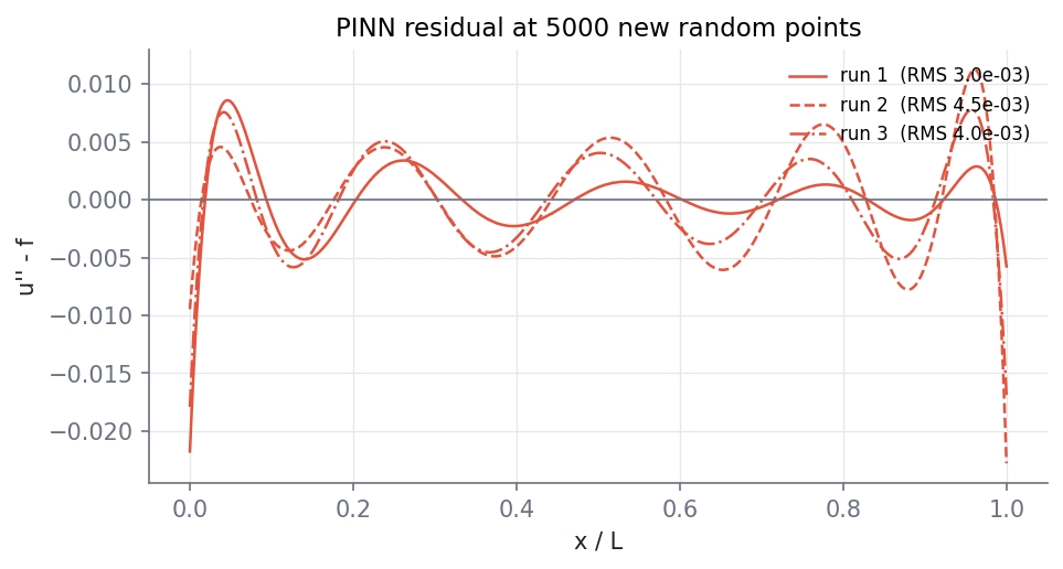
Figure 6. The residual $u'' - f$ at 5000 random points that were not used in training.
The residual is how far the trained network is from satisfying the equation. At points it never saw, its root-mean-square is $3.0 \times 10^{-3}$ to $4.5 \times 10^{-3}$, against a source term that reaches 9.6: a few parts in ten thousand. It is largest at the two ends, where the moment and shear errors are largest too.
The FEM reference, checked
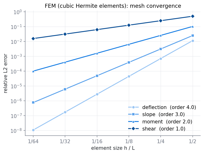
Figure 7. FEM error against element size, from 2 to 64 elements.
A reference is only useful if it is right. The FEM errors fall at exactly the rates theory predicts for cubic elements: order 4 for the deflection, 3 for the slope, 2 for the moment and 1 for the shear. The nodal deflections are exact at every mesh, to round-off. Beyond about 64 elements, round-off starts to dominate, because the stiffness matrix of a beam becomes ill-conditioned as the elements shrink.
7. What to take away
- Reduce the order when the physics allows it. A statically determinate beam needs only $EI\,w'' = -M(x)$, a Poisson problem the Studio solves directly.
- Check derived quantities, not just the field. The deflection was accurate to about $10^{-5}$. The shear, from the third derivative, was off by up to about 6 %, and most at the supports.
- Run more than once. Three runs from different starting weights gave deflection errors from $7.9 \times 10^{-6}$ to $1.5 \times 10^{-5}$. Your run will land somewhere in that range, not on one of these numbers.
- Compare with care. Say which mesh, which equation and which way of computing derived quantities each method used. Otherwise "PINN vs FEM" means little.
All results on this page are from three runs on one machine, with the default network and Adam followed by L-BFGS.
Try next
- Change the load to $q(x) = q_0\,x/L$ (a triangular load). Statics still gives $M(x)$, so the Studio can still solve it. Work out the new source term and exact solution.
- A cantilever (clamped at $x = 0$, free at $x = L$) is also statically determinate. Its two conditions, $w(0) = 0$ and $w'(0) = 0$, are both at the same end. Can you set that up in the Studio?
- A beam clamped at both ends is statically indeterminate. It needs the full fourth-order equation, which the Studio cannot express yet.
Files
beam_compare.py
- beam_compare.py: the comparison script (NumPy, SciPy, Matplotlib; PyTorch to load the network).