Why PINN losses are hard

Section 3.2 showed that the speed of gradient descent is set by the condition number of the loss, the ratio of its largest curvature to its smallest: the step must be small enough for the steepest direction, and progress along the flattest is then slow. This section shows that PINN losses are badly conditioned for a reason that can be computed exactly, and what that does to the training of a network.

A model that can be solved exactly

Take as the trial function a sum of sines, $u(x) = \sum_{j=1}^{J} c_j \sin(j\pi x)$ on $[0, 1]$, with the coefficients $c_j$ as the parameters. It satisfies $u(0) = u(1) = 0$ whatever they are, so only one loss term remains. Fitting values, the loss is the mean of $(u - u^\ast)^2$. Fitting the equation $-u'' = f$, it is the mean of $(-u'' - f)^2$, and since $-u'' = \sum_j c_j (j\pi)^2\sin(j\pi x)$, each coefficient now enters multiplied by $(j\pi)^2$. Both losses are quadratic in the coefficients, so their Hessians are constant matrices:

import numpy as np

x = np.linspace(0, 1, 4001)[1:-1]                       # a fine grid inside (0, 1)
for J in (4, 8, 16):
    j = np.arange(1, J + 1)
    values = np.sin(np.pi * np.outer(x, j))              # column j: the j-th sine at every point
    second = (np.pi * j) ** 2 * values                   # -u'' of each sine
    H_values = 2 * values.T @ values / len(x)            # Hessian of the mean of (u - u*)^2
    H_equation = 2 * second.T @ second / len(x)          # Hessian of the mean of (-u'' - f)^2
    print(f"J = {J:2d}:  condition number fitting values {np.linalg.cond(H_values):5.2f},"
          f"  fitting the equation {np.linalg.cond(H_equation):7.0f}   (J^4 = {J**4})")

J =  4:  condition number fitting values  1.00,  fitting the equation     256   (J^4 = 256)
J =  8:  condition number fitting values  1.00,  fitting the equation    4096   (J^4 = 4096)
J = 16:  condition number fitting values  1.00,  fitting the equation   65536   (J^4 = 65536)

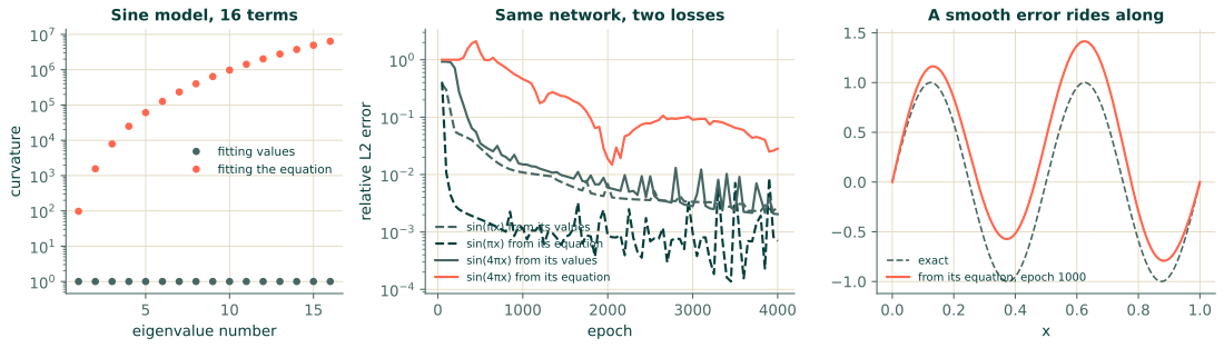
Fitting values is perfectly conditioned, because the sines are orthogonal. Fitting the equation multiplies the curvature in the direction of the $j$-th sine by $(j\pi)^4$, and the condition number grows like $J^4$. The reason is general. Minimising $\|A\mathbf{c} - \mathbf{b}\|^2$ has Hessian $2A^\top A$, whose condition number is the square of $A$'s, and a differential operator of order $m$ stretches a component of wavenumber $j$ by about $j^m$. A least-squares residual loss therefore stretches it by $j^{2m}$: $j^4$ for Poisson's equation, $j^8$ for the beam of Section 8.5. It is the same squaring that made the normal equations of Section 1.3 ill-conditioned.

Dividing the residual by a constant, as Section 4.5 taught, scales every curvature by the same factor and leaves the condition number alone. Scaling balances one term against another; it does nothing to the conditioning within a term.

What it does to a network

A network is not a sum of sines, but the operator does the same to it. Here the same network learns the same two functions twice, once from their values and once from their equation, $-u'' = k^2\sin(kx)$ with $u(0) = u(1) = 0$, residual divided by $k^2$; three seeds each, the middle error after a given number of epochs:

import math
import torch
import torch.nn as nn

def d(y, x):
    return torch.autograd.grad(y, x, torch.ones_like(y), create_graph=True)[0]

x_test = torch.linspace(0, 1, 2001).reshape(-1, 1)
checkpoints = (250, 500, 1000, 2000, 4000)

def learn(m, source, seed, epochs=4000):
    """Learn sin(m pi x) from its values or from its equation; the error at each checkpoint."""
    k = m * math.pi
    exact = lambda x: torch.sin(k * x)
    torch.manual_seed(seed)
    net = nn.Sequential(nn.Linear(1, 32), nn.Tanh(), nn.Linear(32, 32), nn.Tanh(),
                        nn.Linear(32, 32), nn.Tanh(), nn.Linear(32, 1))
    u = lambda x: net(2 * x - 1)
    x = torch.rand(128, 1)
    x_b = torch.tensor([[0.0], [1.0]])
    opt = torch.optim.Adam(net.parameters(), lr=1e-3)
    errors = []
    for epoch in range(1, epochs + 1):
        opt.zero_grad()
        if source == "values":
            loss = ((u(x) - exact(x)) ** 2).mean()
        else:
            xg = x.clone().requires_grad_(True)
            residual = (-d(d(u(xg), xg), xg) - k**2 * exact(xg)) / k**2
            loss = (residual ** 2).mean() + (u(x_b) ** 2).sum()
        loss.backward()
        opt.step()
        if epoch in checkpoints:
            with torch.no_grad():
                errors.append(((u(x_test) - exact(x_test)).norm() / exact(x_test).norm()).item())
    return errors

print("relative L2 error after epochs:          " + "  ".join(f"{c:7d}" for c in checkpoints))
for m in (1, 4):
    for source in ("values", "equation"):
        runs = [learn(m, source, seed) for seed in range(3)]
        middle = [sorted(run[i] for run in runs)[1] for i in range(len(checkpoints))]
        print(f"sin({m} pi x) from its {source:8s}               " + "  ".join(f"{e:7.1e}" for e in middle))

relative L2 error after epochs:              250      500     1000     2000     4000
sin(1 pi x) from its values                 5.1e-02  2.9e-02  1.1e-02  6.9e-03  2.8e-03
sin(1 pi x) from its equation               2.5e-03  1.7e-03  1.2e-03  8.7e-04  7.0e-04
sin(4 pi x) from its values                 2.7e-01  3.5e-02  1.5e-02  5.9e-03  2.0e-03
sin(4 pi x) from its equation               1.0e+00  1.3e+00  4.6e-01  1.9e-02  2.8e-02

For $\sin(\pi x)$ the equation is the better teacher: after 250 epochs its error is twenty times smaller than the fit to values, and it stays ahead. For $\sin(4\pi x)$ the order reverses. The fit to values is at 3.5% after 500 epochs; the PINN is still at 100% or worse, and after 4000 epochs it is fourteen times less accurate than the fit. The network, the optimiser and the function are the same; only the loss differs.

Long wavelengths are almost free

The exact model says why. Measure what an error costs: add 0.4 times a sine to the exact solution of the $\sin(4\pi x)$ problem, once with a long wavelength and once with the solution's own, and evaluate both losses:

k = 4 * math.pi
xg = torch.linspace(0, 1, 2001)[1:-1].reshape(-1, 1).requires_grad_(True)
for name, error in [("smooth error 0.4 sin(pi x)       ", lambda x: 0.4 * torch.sin(math.pi * x)),
                    ("same wavelength, 0.4 sin(4 pi x) ", lambda x: 0.4 * torch.sin(k * x))]:
    u = torch.sin(k * xg) + error(xg)
    residual = (-d(d(u, xg), xg) - k**2 * torch.sin(k * xg)) / k**2
    print(f"{name} costs {(error(xg) ** 2).mean().item():.1e} in the values loss,"
          f" {(residual ** 2).mean().item():.1e} in the equation loss")

smooth error 0.4 sin(pi x)        costs 8.0e-02 in the values loss, 3.1e-04 in the equation loss
same wavelength, 0.4 sin(4 pi x)  costs 8.0e-02 in the values loss, 8.0e-02 in the equation loss

To the values loss the two errors are the same. To the equation loss the smooth one is $4^4 = 256$ times cheaper: once a network has the oscillation right, a smooth error of 40% adds only $3\times10^{-4}$ to its loss. The loss surface is nearly flat in the direction that would remove such an error, so a method that follows its slope moves slowly that way. Figure 9.1 (right) shows the seed-0 run at epoch 1000: the oscillation is in place, riding on a smooth hump that the loss barely notices.

What this means for the choice of optimiser

• Gradient descent must keep its step below the stiffest curvature and then crawls along the flattest (Section 3.2). With a condition number growing like $J^4$, that is hopeless for any solution with detail.
• Adam rescales each parameter by the size of its own gradient (Section 3.5). The slow directions here are smooth changes of the function $u$, which involve many parameters at once, so Adam helps, but much less than in Section 3.5's toy problem, where the stiff directions lay along the parameters. Section 9.2 gets the most out of it.
• Methods that use curvature undo the conditioning instead of suffering it. On the sine model, one Newton or Gauss–Newton step solves the problem exactly, whatever $J$. L-BFGS (Section 9.3) builds an approximation to the curvature from the gradients it has seen; Gauss–Newton methods (Section 9.4) compute it.

Rathore et al. (2024) studied the loss landscapes of PINNs for several equations and reached the same conclusion: the differential operator makes the loss ill-conditioned, Adam alone or L-BFGS alone each stall, and Adam followed by L-BFGS, or by a Newton-type method, trains better than either.

Exercises

1. In the sine model, what is the condition number of the equation loss for the beam equation, $w'''' = q$, with $J$ terms? What does that suggest about the two formulations of Section 8.5?
2. In the network experiment, learning $\sin(\pi x)$ from its equation was faster than from its values. Using the cost of errors, explain why.
3. Halving the learning rate of plain gradient descent on the sine model makes every step safer. Why does it not help with the condition number?

Recap

• A least-squares residual loss squares the differential operator: in a sine basis its condition number grows like $J^4$ for a second-order equation, against 1 for fitting values.
• Long-wavelength errors are nearly free in the residual loss, so a PINN can hold a smooth error for a long time, and scaling the residual does not change that.
• First-order methods suffer the conditioning; methods that use curvature, from L-BFGS to Gauss–Newton, are designed to remove it.

References

- Rathore, P., Lei, W., Frangella, Z., Lu, L., & Udell, M. (2024). Challenges in training PINNs: A loss landscape perspective. Proceedings of the 41st International Conference on Machine Learning, 235, 42159–42191. https://proceedings.mlr.press/v235/rathore24a.html