Gradient-based balancing

Fixed weights from the scales (Section 10.2) need the scales. When they are hard to estimate, the weights can be set from the training itself. Wang et al. (2021) measured the gradients of each loss term layer by layer during training and found that the equation term's gradients were often orders of magnitude larger than the boundary term's, so that the boundary was neglected: Section 10.1's first failure, seen from inside the optimiser. They called this a gradient pathology, and proposed to fix it by adjusting the boundary weight as training goes on.

Learning-rate annealing

Every few steps (every 10 in their experiments), estimate the weight that would bring the boundary term's typical gradient up to the size of the equation term's largest one,

$$\hat w_b = \frac{\max_\theta \bigl|\nabla_\theta L_r\bigr|}{\operatorname{mean}_\theta \bigl|\nabla_\theta L_b\bigr|},$$

the maximum and the mean taken over all the parameters, and move the weight towards it, $w_b \leftarrow (1 - \alpha)\,w_b + \alpha\,\hat w_b$, with $\alpha = 0.9$ recommended.

There is a feedback loop in this rule, and it points the wrong way. As the boundary is met, $L_b$ and its gradient shrink, so $\hat w_b$ grows; a larger weight meets the boundary more closely, which shrinks its gradient further. Nothing stops the weight, and Section 10.1 showed where a huge boundary weight leads: to $u = 0$, which meets the boundary perfectly. Measure the boundary term's gradient with its current weight instead, and the estimate becomes $\hat w_b = \max|\nabla L_r| \big/ \bigl(w_b\operatorname{mean}|\nabla L_b|\bigr)$: a larger weight lowers its own estimate. The update then has a fixed point, where $w_b = \hat w_b$, that is

$$w_b^\ast = \sqrt{\frac{\max_\theta|\nabla_\theta L_r|}{\operatorname{mean}_\theta|\nabla_\theta L_b|}},$$

and the weight settles near it instead of running away. We call this the self-limiting form.

The experiment

The test is the paper's own benchmark: the Helmholtz equation $u_{xx} + u_{yy} + u = q$ on $[-1, 1]^2$, with $u = 0$ on the boundary and the source chosen so that $u = \sin(\pi x)\sin(4\pi y)$. As in the paper: four hidden layers of 50 tanh neurons with Glorot initialisation, Adam at $10^{-3}$, and fresh random batches of 128 interior and 128 boundary points at every step; 10000 steps here, against the paper's 40000.

import math
import torch
import torch.nn as nn

def d(y, x):
    return torch.autograd.grad(y, x, torch.ones_like(y), create_graph=True)[0]

exact = lambda p: torch.sin(math.pi * p[:, :1]) * torch.sin(4 * math.pi * p[:, 1:])
q = lambda p: (1 - math.pi**2 - (4 * math.pi) ** 2) * exact(p)          # u_xx + u_yy + u = q

def on_boundary(n, g):                                  # n random points on the edges of [-1, 1]^2
    s = 2 * torch.rand(n, 1, generator=g) - 1
    side = torch.randint(0, 4, (n, 1), generator=g)
    x = torch.where(side == 0, -1.0, torch.where(side == 1, 1.0, s))
    y = torch.where(side == 2, -1.0, torch.where(side == 3, 1.0, s))
    return torch.cat([x, y], dim=1)

ticks = torch.linspace(-1, 1, 101)
grid = torch.stack(torch.meshgrid(ticks, ticks, indexing="ij"), dim=-1).reshape(-1, 2)

def train(scheme, seed, epochs=10000, every=10, alpha=0.9):
    g = torch.Generator().manual_seed(seed)
    torch.manual_seed(seed)
    layers = [nn.Linear(2, 50), nn.Linear(50, 50), nn.Linear(50, 50), nn.Linear(50, 50), nn.Linear(50, 1)]
    for layer in layers:                                # Glorot initialisation, as in the paper
        nn.init.xavier_normal_(layer.weight)
        nn.init.zeros_(layer.bias)
    net = nn.Sequential(layers[0], nn.Tanh(), layers[1], nn.Tanh(), layers[2], nn.Tanh(),
                        layers[3], nn.Tanh(), layers[4])
    params = list(net.parameters())
    opt = torch.optim.Adam(params, lr=1e-3)
    w_b, history = 1.0, []
    for epoch in range(epochs):
        p = (2 * torch.rand(128, 2, generator=g) - 1).requires_grad_(True)
        u = net(p)
        grad_u = d(u, p)
        lap = d(grad_u[:, :1], p)[:, :1] + d(grad_u[:, 1:], p)[:, 1:]
        loss_r = ((lap + u - q(p)) ** 2).mean()
        loss_b = (net(on_boundary(128, g)) ** 2).mean()
        if scheme != "fixed" and epoch % every == 0:
            g_r = torch.autograd.grad(loss_r, params, retain_graph=True, allow_unused=True)
            term_b = w_b * loss_b if scheme == "self-limiting" else loss_b
            g_b = torch.autograd.grad(term_b, params, retain_graph=True)
            w_hat = max(t.abs().max() for t in g_r if t is not None) / torch.cat([t.abs().flatten() for t in g_b]).mean()
            w_b = (1 - alpha) * w_b + alpha * w_hat.item()
        history.append(w_b)
        opt.zero_grad()
        (loss_r + w_b * loss_b).backward()
        opt.step()
    with torch.no_grad():
        error = ((net(grid) - exact(grid)).norm() / exact(grid).norm()).item()
    return error, history

print("scheme           relative L2 error (2 seeds)    boundary weight over the last 5000 steps")
for scheme in ("fixed", "as printed", "self-limiting"):
    for seed in range(2):
        error, history = train(scheme, seed)
        late = history[5000:]
        print(f"{scheme:14s}   seed {seed}: {error:.1e}             between {min(late):.1e} and {max(late):.1e}")

scheme           relative L2 error (2 seeds)    boundary weight over the last 5000 steps
fixed            seed 0: 3.8e-01             between 1.0e+00 and 1.0e+00
fixed            seed 1: 8.2e-01             between 1.0e+00 and 1.0e+00
as printed       seed 0: 1.0e+00             between 4.5e+04 and 1.9e+09
as printed       seed 1: 1.0e+00             between 1.5e+04 and 2.5e+09
self-limiting    seed 0: 4.5e-02             between 9.8e+01 and 3.0e+03
self-limiting    seed 1: 1.2e-01             between 1.2e+02 and 3.4e+03

With equal weights the errors are 38% and 82%; the paper, with four times as many steps and a decaying learning rate, reports about 16 to 18% for this case. As printed, the rule sends the boundary weight beyond $10^4$, and on to $10^9$ in the second half of training, and both runs end at $u = 0$: an error of exactly 100%. The self-limiting form keeps the weight between about 100 and 3000 and brings the error down to 4.5% and 12%, seven to eight times smaller than with fixed weights. The paper's own figure for this problem shows its weight settling between about 50 and 350: the behaviour of a rule with a fixed point, not of one that runs away. With 40000 steps the paper reached 1.3%; the 10000 constant-rate steps here are a quarter of that budget.

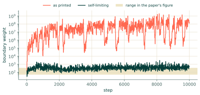
Weights that feed on their own success

The runaway is not special to this rule. Any scheme that raises a term's weight because the term has become small, rather than because it is being neglected, has the same loop. The simplest such scheme divides each term by its own current value, so that every term counts as 1: as a condition is met, its value falls and its weight rises without limit. A safe adaptive scheme has a fixed point, or a cap, and its weights are worth plotting: a weight that keeps climbing for the whole run is a warning, not a result.

In the Studio

The Loss block's Weighting scheme offers Fixed only. Its menu lists Normalised by term magnitude and Gradient-norm balancing as coming later; the first of these is the self-feeding scheme described above, and either needs a fixed point or a cap before it is safe. A generated script can be given a balancing scheme by replacing its Balancer class, whose update(epoch, terms) method the training loop calls after every step and whose weights it multiplies each group of terms by.

Exercises

1. Derive the fixed point $w_b^\ast$ of the self-limiting update, assuming the two gradient statistics change slowly.
2. Why does the estimate use the largest gradient of the equation term but the mean gradient of the boundary term?
3. The weight is updated every 10 steps and smoothed with $\alpha = 0.9$. What would go wrong if it were set to $\hat w_b$ at every step, with no smoothing, in a run with fresh random points at every step?

Recap

• Learning-rate annealing sets the boundary weight from the ratio of the terms' gradients, an automatic version of balancing by scales.
• Read literally, the rule feeds on its own success: in our runs the weight ran away and the network went to the trivial solution. Measuring the boundary gradient with its current weight gives a fixed point, and that form improved the benchmark's error several times over.
• Scale first, adapt second, and plot the weights.

References

- Wang, S., Teng, Y., & Perdikaris, P. (2021). Understanding and mitigating gradient flow pathologies in physics-informed neural networks. SIAM Journal on Scientific Computing, 43(5), A3055–A3081. doi:10.1137/20M1318043