Fourier features

Section 9.1 met one reason a PINN is slow on solutions with detail: the residual loss is badly conditioned. A second reason lies in the network itself. Trained by gradient descent, networks fit the smooth, long-wavelength part of a function first and its fine detail much later: their spectral bias (Rahaman et al., 2019). For a solution with several scales the fine scale can be left out for the whole of a training run.

Lifting the input

Tancik et al. (2020) proposed a simple remedy. Before the first layer, replace the input $z$ (scaled to $[-1, 1]$) by sines and cosines of it at random frequencies,

$$\gamma(z) = \bigl(\sin(2\pi b_1 z), \dots, \sin(2\pi b_m z), \cos(2\pi b_1 z), \dots, \cos(2\pi b_m z)\bigr), \qquad b_j \sim \mathcal{N}(0, \sigma^2),$$

and let the network work on $\gamma(z)$. The frequencies are drawn once and then fixed. A feature with frequency $b$ completes $2b$ periods across the domain, so a network fed such features can produce oscillations of that order from its first layer instead of having to build them from scratch. The width $\sigma$ sets which frequencies are on offer.

Two scales in one solution

The test has a large, slow part and a small, fast one, ten periods across the interval:

$$-u'' = f \ \text{ on } (0, 1), \qquad u(x) = \sin(2\pi x) + 0.1\sin(20\pi x), \qquad u(0) = u(1) = 0,$$

with the residual divided by the size of $f$, about 430 (Section 10.2). Four networks, all with three hidden layers of 32 tanh neurons and 32 random frequencies where they have any: plain; Fourier features with $\sigma = 1$, 5 and 20; and multi-scale, half the frequencies with $\sigma = 1$ and half with $\sigma = 5$, an idea of Wang et al. (2021) for solutions with several scales:

import math
import torch
import torch.nn as nn

def d(y, x):
    return torch.autograd.grad(y, x, torch.ones_like(y), create_graph=True)[0]

exact = lambda x: torch.sin(2 * math.pi * x) + 0.1 * torch.sin(20 * math.pi * x)
f = lambda x: (2 * math.pi) ** 2 * torch.sin(2 * math.pi * x) + 0.1 * (20 * math.pi) ** 2 * torch.sin(20 * math.pi * x)
f_size = (2 * math.pi) ** 2 + 0.1 * (20 * math.pi) ** 2
x_test = torch.linspace(0, 1, 4001).reshape(-1, 1)

class FourierFeatures(nn.Module):
    def __init__(self, sigmas, m, generator):
        super().__init__()
        B = torch.cat([s * torch.randn(1, m // len(sigmas), generator=generator) for s in sigmas], dim=1)
        self.register_buffer("B", B)                         # drawn once, never trained
    def forward(self, z):
        p = 2 * math.pi * z @ self.B
        return torch.cat([torch.sin(p), torch.cos(p)], dim=1)

def train(sigmas, seed, epochs=5000, m=32, width=32):
    generator = torch.Generator().manual_seed(1000 + seed)
    torch.manual_seed(seed)
    encode = FourierFeatures(sigmas, m, generator) if sigmas else nn.Identity()
    net = nn.Sequential(encode, nn.Linear(2 * m if sigmas else 1, width), nn.Tanh(),
                        nn.Linear(width, width), nn.Tanh(), nn.Linear(width, width), nn.Tanh(), nn.Linear(width, 1))
    u = lambda x: net(2 * x - 1)
    x = torch.rand(400, 1).requires_grad_(True)
    x_b = torch.tensor([[0.0], [1.0]])
    opt = torch.optim.Adam(net.parameters(), lr=1e-3)
    for epoch in range(epochs):
        opt.zero_grad()
        loss = (((-d(d(u(x), x), x) - f(x)) / f_size) ** 2).mean() + (u(x_b) ** 2).mean()
        loss.backward()
        opt.step()
    x_fresh = torch.rand(4000, 1, generator=torch.Generator().manual_seed(7)).requires_grad_(True)
    held_out = (((-d(d(u(x_fresh), x_fresh), x_fresh) - f(x_fresh)) / f_size) ** 2).mean().item()
    with torch.no_grad():
        error = ((u(x_test) - exact(x_test)).norm() / exact(x_test).norm()).item()
    return error, loss.item(), held_out

print("network                       relative L2 error (2 seeds)   training loss     loss at fresh points")
for name, sigmas in [("plain", []), ("Fourier features, sigma 1", [1.0]), ("Fourier features, sigma 5", [5.0]),
                     ("Fourier features, sigma 20", [20.0]), ("multi-scale, sigma 1 and 5", [1.0, 5.0])]:
    runs = [train(sigmas, seed) for seed in range(2)]
    print(f"{name:28s}  " + "  ".join(f"{r[0]:.1e}" for r in runs) + "        "
          + "  ".join(f"{r[1]:.0e}" for r in runs) + "     " + "  ".join(f"{r[2]:.0e}" for r in runs))

network                       relative L2 error (2 seeds)   training loss     loss at fresh points
plain                         8.9e-02  3.7e-01        3e-04  4e-02     6e-04  5e-02
Fourier features, sigma 1     1.1e-02  1.1e-02        5e-06  2e-04     6e-06  2e-05
Fourier features, sigma 5     2.7e-01  1.3e-01        6e-07  2e-06     3e-03  3e-03
Fourier features, sigma 20    1.0e+00  1.0e+00        5e-05  2e-04     2e+00  2e+00
multi-scale, sigma 1 and 5    7.3e-03  4.9e-02        7e-07  7e-07     8e-07  2e-05

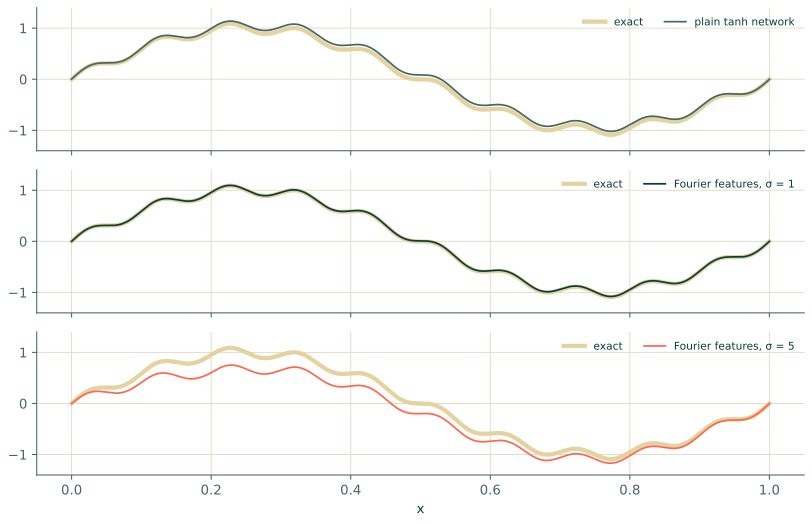
With $\sigma = 1$, the Studio's default, the error is 1.1% in both runs, eight and thirty times smaller than the plain network's. Faster features are worse, and the last two columns say why. With $\sigma = 5$ the training loss is the smallest in the table, below $10^{-6}$, while the loss at fresh points is a thousand times larger or more: the network has satisfied the equation at its 400 points and not between them. With $\sigma = 20$ the same happens on a larger scale, and the error is 100%. The multi-scale network was the best of all in one run, 0.7%, and fair in the other, 4.9%, where its loss at fresh points is thirty times its training loss: mixing scales helps when both are needed, and brings some of the fast features' trouble with it. The lesson is less "use Fourier features" than "choose their frequencies, and check between the points".

Choosing the frequencies

• Match $\sigma$ to the solution. On the scaled input $z \in [-1, 1]$, a component with $n$ periods across the domain needs frequencies of about $n/2$. Start near 1, the Studio's default, and raise it only for a solution known to oscillate quickly; the frequencies $\sigma$ offers become the frequencies the network finds easy, and the others become harder (the eigenvector bias of Wang et al. (2021)).
• Too high is worse than too low. Features faster than the solution can fit the collocation points with oscillations between them, the aliasing of Section 6.1: check the residual at fresh points (Section 6.5).
• For a periodic solution, use exact features. On a domain of length $P$ with periodic conditions, feed the network $\cos(2\pi x/P)$ and $\sin(2\pi x/P)$ (and their multiples) instead of $x$: every function of them is periodic, so the condition holds exactly and leaves the loss (Dong & Ni, 2021).
• Fix the random frequencies with a seed. They are part of the network; a different draw is a different network.

In the Studio

Connect an Encoding block between the Domain and the Network and choose Mapping Fourier features, with Fourier features (the number $m$, default 32) and Fourier sigma ($\sigma$, default 1.0); Normalise inputs to [-1, 1] applies the scaling of Section 11.1 first. The generated script uses the same form as above, 2π z B. Its matrix B is drawn when the network is built, which happens when the script is loaded and before train() seeds the random generator (the seeding order noted in Section 13.1). Until the generator changes, seed PyTorch yourself before loading the script if you want the same frequencies in every run.

Exercises

1. How many periods across the domain does a feature with $b = 3$ have? Which frequencies does $u = \sin(2\pi x) + 0.1\sin(20\pi x)$ need?
2. With $\sigma = 5$, about what fraction of the 32 frequencies have $|b| < 0.5$? Why does that matter here?
3. A solution is periodic in $x$ with period 1 and smooth. Which encoding would you use, and what does it do to the loss?

Recap

• Networks have a spectral bias: smooth parts first, fine detail late. Fourier features change which frequencies come easily.
• On a two-scale solution, features of width $\sigma = 1$ beat a plain network eight to thirty times over; features much faster than the solution fitted the collocation points and nothing between them.
• Choose $\sigma$ from the frequencies the solution needs, seed the draw, and use exact periodic features when the problem is periodic.

References

- Dong, S., & Ni, N. (2021). A method for representing periodic functions and enforcing exactly periodic boundary conditions with deep neural networks. Journal of Computational Physics, 435, 110242. doi:10.1016/j.jcp.2021.110242
- Rahaman, N., Baratin, A., Arpit, D., et al. (2019). On the spectral bias of neural networks. Proceedings of the 36th International Conference on Machine Learning, 97, 5301–5310. https://proceedings.mlr.press/v97/rahaman19a.html
- Tancik, M., Srinivasan, P. P., Mildenhall, B., et al. (2020). Fourier features let networks learn high frequency functions in low dimensional domains. Advances in Neural Information Processing Systems, 33, 7537–7547. https://proceedings.neurips.cc/paper_files/paper/2020/hash/55053683268957697aa39fba6f231c68-Abstract.html
- Wang, S., Wang, H., & Perdikaris, P. (2021). On the eigenvector bias of Fourier feature networks: From regression to solving multi-scale PDEs with physics-informed neural networks. Computer Methods in Applied Mechanics and Engineering, 384, 113938. doi:10.1016/j.cma.2021.113938