Reading the loss curves
A total loss that falls tells you almost nothing. Plotted term by term, with the residual at fresh points beside it, the same curves tell you which of half a dozen things has gone wrong.
Section 3.2 warned that a loss that stops falling is not necessarily a solution, and Section 6.2 that a loss that falls is not necessarily one either. This section trains the same small PINN six times: once as it should be, once on a harder version of the problem, and four times with one setting wrong. It shows what each looks like in the only evidence you have when no reference solution exists: the loss of each term over the epochs, and the residual at points the network was not trained on.
Six runs
The problem is $-u'' = k^2\sin(kx)$ on $(0, 1)$ with $u(0) = u(1) = 0$, whose solution $\sin(kx)$ is known, so each run can be graded afterwards. The runs differ in one setting each:
| Run | $k$ | Residual | Boundary weight | Learning rate | Points |
|---|---|---|---|---|---|
| healthy | $\pi$ | divided by $k^2$ | 1 | $10^{-3}$ | 64 |
| harder problem | $4\pi$ | divided by $k^2$ | 1 | $10^{-3}$ | 128 |
| boundary too light | $4\pi$ | as written | 1 | $10^{-3}$ | 128 |
| boundary too heavy | $4\pi$ | as written | $10^8$ | $10^{-3}$ | 128 |
| step too large | $4\pi$ | divided by $k^2$ | 1 | $10^{-2}$ | 128 |
| too few points | $4\pi$ | divided by $k^2$ | 1 | $10^{-3}$ | 8 |
import math
import torch
import torch.nn as nn

def d(y, x):
    return torch.autograd.grad(y, x, torch.ones_like(y), create_graph=True)[0]

def run(k, scaled, w_b, lr, n_points, seed=0, epochs=4000):
    torch.manual_seed(seed)
    net = nn.Sequential(nn.Linear(1, 32), nn.Tanh(), nn.Linear(32, 32), nn.Tanh(),
                        nn.Linear(32, 32), nn.Tanh(), nn.Linear(32, 1))
    u = lambda x: net(2 * x - 1)
    scale = k**2 if scaled else 1.0
    residual = lambda x: (-d(d(u(x), x), x) - k**2 * torch.sin(k * x)) / scale
    x = torch.rand(n_points, 1).requires_grad_(True)
    x_b = torch.tensor([[0.0], [1.0]])
    opt = torch.optim.Adam(net.parameters(), lr=lr)
    history = {"equation": [], "boundary": []}
    for epoch in range(epochs):
        opt.zero_grad()
        loss_r, loss_b = (residual(x) ** 2).mean(), (u(x_b) ** 2).mean()
        (loss_r + w_b * loss_b).backward()
        opt.step()
        history["equation"].append(loss_r.item())
        history["boundary"].append(loss_b.item())
    x_fresh = torch.rand(2000, 1, generator=torch.Generator().manual_seed(99)).requires_grad_(True)
    fresh = (residual(x_fresh) ** 2).mean().item()
    x_test = torch.linspace(0, 1, 2001).reshape(-1, 1)
    with torch.no_grad():
        error = ((u(x_test) - torch.sin(k * x_test)).norm() / torch.sin(k * x_test).norm()).item()
        size = u(x_test).abs().max().item()
    return history, fresh, error, size

k4 = 4 * math.pi
runs = {"healthy": (math.pi, True, 1, 1e-3, 64), "harder problem": (k4, True, 1, 1e-3, 128),
        "boundary too light": (k4, False, 1, 1e-3, 128), "boundary too heavy": (k4, False, 1e8, 1e-3, 128),
        "step too large": (k4, True, 1, 1e-2, 128), "too few points": (k4, True, 1, 1e-3, 8)}
results = {name: run(*settings) for name, settings in runs.items()}

print("run                  equation term          boundary term      jumps   fresh/trained   error   largest |u|")
print("                     start      end         start     end      (x)     residual")
for name, (h, fresh, error, size) in results.items():
    eq, bc = h["equation"], h["boundary"]
    tail = eq[-400:]
    jumps = max(tail) / min(tail)
    print(f"{name:19s}  {eq[0]:8.1e}  {eq[-1]:8.1e}    {bc[0]:8.1e}  {bc[-1]:8.1e}  {jumps:6.0f}   {fresh / eq[-1]:9.1e}"
          f"   {error:6.1e}  {size:6.2f}")
run                  equation term          boundary term      jumps   fresh/trained   error   largest |u|
                     start      end         start     end      (x)     residual
healthy               4.7e-01   1.1e-06     2.8e-02   8.6e-08       8     8.3e-01   2.5e-04    1.00
harder problem        5.1e-01   1.4e-05     2.8e-02   8.0e-05       2     2.1e+00   1.2e-02    1.01
boundary too light    1.3e+04   4.6e+00     2.8e-02   3.3e+01       1     1.6e+00   4.7e+00    5.77
boundary too heavy    1.3e+04   1.3e+04     2.8e-02   3.8e-13       1     1.0e+00   1.0e+00    0.02
step too large        5.1e-01   8.9e-05     2.8e-02   2.7e-04      31     1.1e+00   1.4e-02    1.01
too few points        5.6e-01   4.7e-09     2.8e-02   8.6e-08  181782     4.3e+07   2.5e+00    2.72
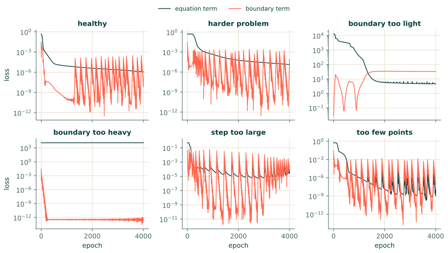
Read the rows against the healthy one: both terms fall by five orders of magnitude or more, the residual at fresh points is about the same as at the training points (a ratio near 1), and the error is $2.5\times10^{-4}$. One feature of Figure 12.1 is common to every run that trains: once the boundary term is very small, it jumps up and down by several orders of magnitude. Adam's steps do not shrink with the gradient (Section 3.5), so a term near $10^{-10}$ is knocked about by steps sized for the equation term. Read a small term by its peaks, not its troughs; in the healthy run even the peaks mean values at the ends of about 0.01.
- Harder problem. Every number looks healthy except the error, 1.2%, and the curves look healthy too: a short flat start, then a fall that slows down without stopping (Figure 12.1). What they cannot show is the smooth error of Section 9.1, which costs the equation term almost nothing. A loss still falling when training stops is the hint; the cures are the optimisers of Chapter 9 and the features of Chapter 11.
- Boundary too light. The equation term falls by a factor of about 3000 while the boundary term rises, from 0.03 to 33: the network trades the boundary for the equation, the signature of Section 10.1's light condition. Its output reaches 5.8 where the solution never exceeds 1.
- Boundary too heavy. The boundary term falls to $10^{-13}$ and the equation term does not move at all. The largest output is 0.02: the network has found $u = 0$, the trivial solution.
- Step too large. The terms fall, but in the last 400 epochs the loss still jumps by a factor of 30. The error of this run happens to be fine, 1.4%; the jumps are the warning that the last epoch need not be (Section 9.2).
- Too few points. The lowest losses in the table, $5\times10^{-9}$, and the largest error, 250%. Two numbers betray it: the loss jumping by a factor of nearly 200,000 at the end, as the network balances on eight points, and above all the residual at fresh points, forty million times the training residual.
What to plot, every run
- Every loss term on its own, on a logarithmic scale. Never only the total.
- The residual at fresh points, many more than the training points, evaluated every few hundred epochs or at least at the end.
- The size of the network's output, against the size you expect. Zero, or a constant, is a diagnosis.
- If you weight terms adaptively, the weights.
In the Studio
The generated script logs every term by name at each Log every interval and returns the full history from
train(); the Visualisation block's loss plot shows each term on a logarithmic scale. For the residual at fresh
points, use the Report block on a fine grid with its residual column (Section 6.5).
Exercises
- Suppose two runs both end with the equation term near its starting value. How do you tell, from the curves alone, a run that has found the trivial solution from one that has not started to learn?
- The too few points run reaches the lowest losses of all. Which number in the table exposes it most clearly?
- In the step too large run, would you trust the weights of the final epoch? What would you do instead?
Answers
- Look at the other terms. A run that has found the trivial solution has driven a condition term to almost nothing while the equation term stays put, and its output is near zero everywhere; a run that has not started to learn has every term near its starting value. The last column of the table separates them at once.
- The ratio of the residual at fresh points to the residual at the training points: forty million, where a healthy run has about one.
- No: its loss is still jumping by large factors, and the last epoch may sit on a spike. Keep the weights with the lowest loss, or better, lower the learning rate with a schedule (Section 9.2) so that the last weights are the best ones.
Recap
- Plot each term separately, on a log scale; one flat term among falling ones is the commonest signature of a failed PINN.
- Jumps of large factors in the equation term mean the step is too large; a loss still falling slowly when training stops points to the conditioning of Section 9.1.
- A small training loss with a large residual at fresh points means the network has learned the points, not the equation. It is the one failure the loss curves cannot show.