Failure modes
The ways a PINN fails are few, and each leaves its own traces. A catalogue, from symptom to cause to first remedy, with the section of this book where each was met.
Every chapter of this book has met at least one way for a PINN to go wrong. This section collects them in one place, organised the way you meet them: by what you see. It has no new experiments. Every entry points to the section where the failure was produced on purpose and measured.
From symptom to cause
| What you see | What to check | Likely cause | First remedy | Where |
|---|---|---|---|---|
| Loss falls; answer close to zero | the output's size; which term is stuck | the trivial solution: the term that carries the data (a source, an initial or boundary value) outweighed, or a long time window | scale the problem; weights from the scales; time windows | 4.5, 6.2, 8.2, 10.1 |
| Equation satisfied; boundary or initial values wrong | each condition term on its own | a condition weighted too lightly | weights from the scales | 10.1, 10.2 |
| Error is a constant, or a straight line | the conditions you imposed | the problem has no unique solution | add the missing condition | 6.3 |
| Small training loss; large error | residual at fresh points | too few points, or features too fast for them | more or redrawn points; slower features; held-out check | 6.5, 7.1, 11.2, 11.3 |
| Long plateau near 100% error, then a slow fall | the error's shape: smooth? | ill-conditioning; spectral bias | L-BFGS after Adam; Fourier features; more epochs | 9.1, 9.3, 11.2 |
| Error stuck at about $10^{-2}$ whatever Adam does | loss jitter at the end | the limit of first-order training | L-BFGS; Gauss–Newton in double precision | 9.2, 9.3, 9.4 |
| Loss jumps by large factors; last epoch worse than earlier ones | jitter in the last few hundred epochs | learning rate too large | a decaying schedule; keep the best weights | 3.6, 9.2 |
| A sharp feature smeared out | residual map around it | too few points where it matters | adaptive sampling; self-adaptive weights | 7.2, 10.4 |
| Error concentrated at a corner | the corner's angle | a singular solution | build the singular behaviour into the trial function | 7.3 |
| Error grows with time | the error in successive time windows | propagation failure | time marching; causal weighting | 8.2 |
| Network output far from the solution's size | inputs and outputs in their units | unscaled inputs saturate; unscaled outputs are slow to grow | scale inputs and outputs inside the network | 4.5, 11.1 |
| L-BFGS stops after a few iterations | anything random in the loss | resampled points or boundary points | fix the points for L-BFGS | 9.3 |
| An adaptive weight keeps growing; answer near zero | the weights' history | a scheme that feeds on its own success | a self-limiting form or a cap; scale first | 10.3 |
| Right shape, wrong sign or factor | the residual evaluated on a known solution | a sign or unit error in the equation | test the residual function before training | 12.3 |
| A parameter estimate that depends on where it started | sensitivity of the data to it | the data cannot determine it | different data, or report it as undetermined | 8.4 |
| Each run gives a different answer | several seeds | an ill-posed problem, or one hard to train | fix the problem first; then report median and range | 6.3, 6.5 |
| NaN | the first epoch at which it appears | a step too large, or a division by zero or a log of a negative number in the trial function | lower the rate; guard the expression | 9.2, 7.3 |
Where to look first
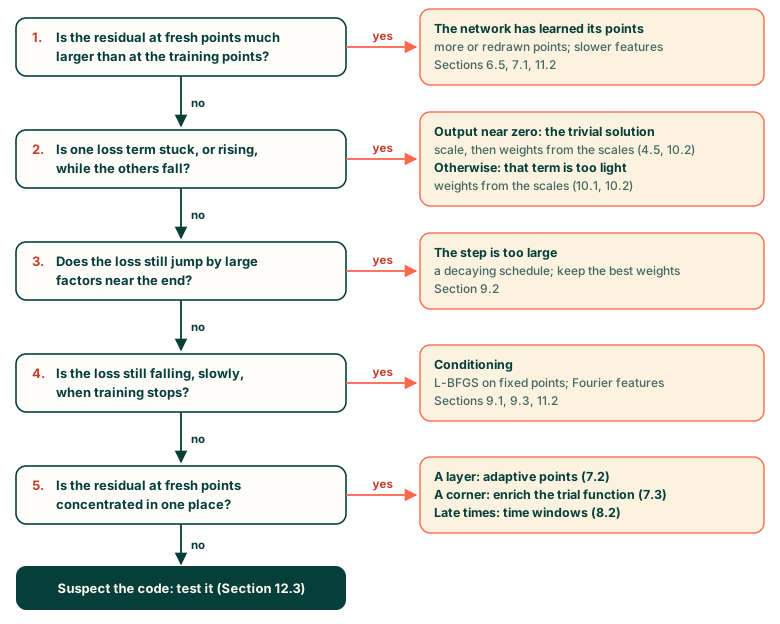
The table is long; the order in which to use it is short. Figure 12.2 puts the questions in the order that separates the commonest failures fastest, using only what a run without a reference solution can show. Its first question is the one the loss curves cannot answer: whether the network has learned the equation or only its training points. Its last box is the subject of the next section.
What the catalogue does not cover
Bugs. A wrong sign in the source, a derivative taken with respect to the wrong variable, a condition imposed at the wrong place: the network trains happily to the solution of a different problem, and every curve looks healthy. The cure is to test the code before training it, which is the subject of the next section.
Exercises
- A run's error is 98%, its output is close to zero everywhere, and its initial-condition term has stayed at about 1 for the whole run while the equation term fell. Which row applies, and what would you try first?
- A 2D run with Second stage: L-BFGS shows almost no improvement in the second stage. What is the first thing to check?
- Why is the residual at fresh points the first question in Figure 12.2, rather than the last?
Answers
- The first row: the trivial solution, with the initial condition outweighed. Scale the equation to its natural units (Sections 4.5 and 6.2) before touching anything else.
- Whether the loss is the same every time it is evaluated: in the Studio's generated script the boundary points are redrawn at each evaluation, which stops L-BFGS within a few iterations (Section 9.3).
- Because it is the one failure that every other diagnostic misses: the loss curves of a network that has learned only its points look better than healthy ones. Ruling it out first means the curves can then be believed.
Recap
- PINN failures are few and recognisable: the trivial solution, a neglected condition, an incomplete problem, points learned instead of the equation, conditioning, step size, sharp or singular features, propagation in time, scaling, and randomness where L-BFGS cannot bear it.
- Check the residual at fresh points first, then each term, then the jitter, then whether the loss is still falling, then where the residual is concentrated.
- None of this catches a bug in the equation itself. Test the residual before training.