Lid-driven cavity: a viscous flow in a box

Poisson and heat problems have one unknown. A fluid has three: two velocity components and a pressure, tied together by three equations. This lesson solves the lid-driven cavity, the standard first test of a flow solver, with a PINN that has three outputs. It then judges the network against a finite element solution, field by field. The network we train (four layers of 50 neurons, tanh) ends with a relative L2 error of 0.23 % in velocity and 0.56 % in pressure.

#studio #navier-stokes #cfd #coupled-equations #fem #validation · 40 min read

Before you start. You should have done Poisson on a square and the Heat in a plate lesson, which introduces the comparison with a finite element reference used here. Open the Studio in another tab. To train the network you need Python with PyTorch and, in practice, a GPU (Colab is one way to get one). To run the reference and the check you need numpy and scipy. The files are listed at the end of this page.

1. The problem

A square box of side 1 is filled with a viscous fluid. The left, right and bottom walls are fixed. The top wall, the lid, slides to the right. How does the fluid move once it has settled?

The unknowns are the horizontal velocity $u$, the vertical velocity $v$ and the pressure $p$, all functions of $(x, y)$. They satisfy the steady incompressible Navier–Stokes equations on $(x, y) \in [0,1]^2$:

$$ u\,u_x + v\,u_y + p_x = \frac{1}{Re}\,(u_{xx} + u_{yy}), \qquad u\,v_x + v\,v_y + p_y = \frac{1}{Re}\,(v_{xx} + v_{yy}), \qquad u_x + v_y = 0 . $$

The first two are momentum balances. The third, continuity, says that the fluid is incompressible. The Reynolds number is $Re = 100$: lid speed 1, box size 1, viscosity $1/Re$. At this value the flow settles to a steady state, which is what these equations describe.

Edge	Condition
Left, $x = 0$	$u = 0$, $v = 0$ (no slip)
Right, $x = 1$	$u = 0$, $v = 0$
Bottom, $y = 0$	$u = 0$, $v = 0$
Lid, $y = 1$	$u = 16\,x^2 (1 - x)^2$, $v = 0$

A smooth lid. The usual benchmark moves the whole lid at speed 1, so the velocity jumps from 0 to 1 at the two top corners. That jump is a singularity that neither a coarse mesh nor a smooth network resolves cleanly, and it would dominate the comparison. Our lid starts at zero at both corners, rises to 1 at the middle and is smooth everywhere, so the comparison measures the network and not the corners. The results below are for this lid, not for the classic one.

Three things to know before computing anything

1. Nothing flows through the walls, so the net flow across any vertical line is zero. In terms of the stream function $\psi$, defined by $u = \psi_y$ and $v = -\psi_x$ with $\psi = 0$ on the bottom wall, this says $\psi = 0$ on all four walls. A network is not told this directly, which makes it a useful check later.
2. The pressure is only defined up to a constant. Only $p_x$ and $p_y$ appear in the equations, so adding a constant to $p$ changes nothing, and there is no boundary condition for $p$. The network is free to choose that constant. Every pressure comparison below is made after subtracting the mean over the cavity, from the network and from the reference alike.
3. The fluid goes round once. The lid drags the fluid to the right, and below it the fluid returns to the left. On the vertical line $x = 0.5$ the horizontal velocity falls from 1 at the lid to a minimum of $-0.163$ at $y = 0.466$ and returns to 0 at the floor. The result is one large clockwise vortex with its centre near $(0.61, 0.75)$. You can see this in the first figure of section 8 before reading a single error.

2. How a PINN sees the problem

The network takes two inputs, $(x, y)$, and gives three outputs, $(u, v, p)$. The loss has eleven terms, each a mean squared residual:

• continuity, $u_x + v_y$,
• the $x$-momentum balance and the $y$-momentum balance (three equation terms),
• $u = 0$ and $v = 0$ on the left, right and bottom walls (six terms),
• $u$ equal to the lid profile and $v = 0$ on the lid (two terms).

Coupled equations and the Studio. As the book explains in section 8.5, a Custom residual block in the Studio can only use its own network output. The momentum equations use $u$, $v$ and $p$ together, so the Studio can build and check this problem, but the residuals in the file it generates are placeholders. The script in this lesson replaces them with the Navier–Stokes residuals. Section 5 lists everything else it changes.

No boundary term for the pressure. The loss has no term that fixes $p$. Its level is set by the equations alone, so the network settles on some constant, and we remove it afterwards.

3. The plan: one block per decision

Block	What it holds
Domain	Rectangle, $x$ and $y$ from 0 to 1, no time dimension
PDE (three blocks)	Elliptic, Custom residual, applied to network output 1, 2 and 3
BC (eight blocks)	Two per wall, one for $u$ (output 1) and one for $v$ (output 2); all Dirichlet
Network	Three outputs, four hidden layers of 50 neurons, tanh
Loss, Optimiser, Train	Fixed equal weights; Adam, then L-BFGS
Visualisation, Report	A field plot with a residual map, a loss curve, a results table

That is 18 blocks and 31 wires.

4. Step by step in the Studio

Step 1: Start a notebook. On the Studio page, name it Lid-driven cavity, choose An empty canvas, and press Create notebook.

Step 2: Place 18 blocks. Domain, three PDE blocks, eight Boundary condition blocks, Network, Loss, Optimiser, Train, Visualisation and Report.

Step 3: Set the Domain. Geometry Rectangle, $x$ from 0 to 1, $y$ from 0 to 1. Leave Time dimension off. Set Interior points to 10000 and Default boundary points to 200. Press Detect boundaries. You should read: BC1 (left), BC2 (right), BC3 (bottom), BC4 (top).

Step 4: Set the three PDE blocks. In each, Equation type Elliptic and Equation Custom residual, with this placeholder:

u_x

Set Applies to network output to 1 in the first block, 2 in the second and 3 in the third. The placeholder only has to be valid. The script replaces it.

Step 5: Set the Network. Network outputs 3, four hidden layers of 50 neurons, activation tanh.

Step 6: Set the eight edge conditions. Each Domain boundary port feeds two BC blocks, one for $u$ and one for $v$. Hover over each port to confirm which edge it is.

Domain port	Edge	Block	Applies to output	Condition type	Value
BC1	left	first	1 ($u$)	Dirichlet	0.0
BC1	left	second	2 ($v$)	Dirichlet	0.0
BC2	right	first	1 ($u$)	Dirichlet	0.0
BC2	right	second	2 ($v$)	Dirichlet	0.0
BC3	bottom	first	1 ($u$)	Dirichlet	0.0
BC3	bottom	second	2 ($v$)	Dirichlet	0.0
BC4	top (lid)	first	1 ($u$)	Dirichlet	16*x**2*(1-x)**2
BC4	top (lid)	second	2 ($v$)	Dirichlet	0.0

Step 7: Set the learning blocks. Leave the Loss at fixed equal weights. In the Optimiser block use Adam at a learning rate of 0.001 and tick Second stage (L-BFGS). In the Train block set 20000 epochs and seed 0.

Step 8: Wire. Press on a dot, drag to a lit dot of the same colour, release. The 31 wires, in order:

1. Domain Coords to each PDE block and to the Network (4 wires)
2. Domain Interior to each PDE block (3 wires)
3. Domain BC1 to BC4 to the eight BC blocks, two for each port (8 wires)
4. The three PDE residuals to Loss, and Network to Loss (4 wires)
5. The eight BC outputs to Loss BC / IC (8 wires)
6. Loss to Train Loss, Optimiser to Train Optimiser (2 wires)
7. Train Model to Visualisation and to Report (2 wires)

Check: the Graph check strip reads nothing to flag. If it complains about the number of network outputs, set the Network to 3 outputs.

Step 9: Generate the code. Press Generate code, then Download .py. This file builds the right problem, with the right points and boundary conditions, but its residuals are the placeholders, so it does not solve the cavity. The next section describes what we change.

What our downloaded file contained. The file we generated for this run had 5,000 epochs, no second stage and the placeholder residuals. The script below sets 20,000 epochs and adds L-BFGS itself, so the results do not depend on what the Studio wrote for those two settings.

5. From the Studio file to the final script

lid_driven_cavity_final.py starts from the Studio file and changes the following. It is self-contained, so you can run it without the Studio file.

• The residuals. The three placeholders become continuity and the two momentum balances, with $Re = 100$.
• The seed. torch.manual_seed is called before the network is built. The Studio file built the network first, so its starting weights changed from run to run.
• The labels. In the Studio file the eight boundary terms carried the same label in pairs (for example "BC1 dirichlet" for both $u$ and $v$ on the left wall), so the loss curves could not tell them apart. The conditions themselves were correct. The loss curves now name each wall and component.
• A second stage. After the Adam epochs, a full-batch L-BFGS stage runs with the boundary points frozen. L-BFGS needs the same objective at every evaluation, and the Studio's boundary points are redrawn at each call.
• Saved output. The field is saved on a 101 × 101 grid every 500 Adam epochs and every 10 L-BFGS rounds (snapshots.npz), and the weights are saved as plain arrays (weights.npz).
• The comparison. The script solves the finite element reference (or loads it from cavity_reference_N128.npz), evaluates the network on a 201 × 201 grid, and writes the metrics, the figures and the GIFs of this page.

Everything else is the Studio's: the network (2 inputs, four hidden layers of 50, three outputs, tanh, Xavier start), 10,000 interior points drawn once, 200 boundary points per wall redrawn at every Adam epoch, all weights equal to 1, Adam at 0.001.

6. Running it

Open a Colab notebook, set the runtime to a GPU, upload lid_driven_cavity_final.py and cavity_reference_N128.npz, and paste the whole script into one cell.

1. Run main(["--smoke"]) first. It trains for 300 epochs on a coarse reference and checks that every step works in about a minute. The numbers it prints mean nothing.
2. Run main(). In our run the Adam stage took 665 s and the L-BFGS stage 261 s, 926 s in all.
3. The script writes cavity_results.zip with the figures, GIFs, metrics and weights. In Colab, download it with from google.colab import files; files.download('cavity_results.zip').

If a figure fails, the script prints a FAILED line and carries on with the rest. With --postprocess-only it reloads model.pt and redoes the comparison without training.

7. The reference solution

We use finite elements: Taylor–Hood elements (biquadratic Q2 velocity, bilinear Q1 pressure) on a uniform mesh of squares, with Newton's method for the nonlinear system. The pressure is fixed at one node, which is why we compare pressures after removing the mean. The solver is in cavity_reference.py and needs only numpy and scipy.

We checked it two ways. First, on Kovasznay flow, a Navier–Stokes solution that is known exactly (here at $Re = 40$ on the unit square). The relative L2 error against the exact solution (python cavity_reference.py --verify):

Elements per side	Velocity error	Order	Pressure error	Order
4	$9.6\times10^{-3}$		$2.7\times10^{-2}$
8	$1.2\times10^{-3}$	3.01	$4.9\times10^{-3}$	2.45
16	$1.5\times10^{-4}$	3.00	$1.2\times10^{-3}$	2.00
32	$1.8\times10^{-5}$	3.02	$3.4\times10^{-4}$	1.85
64	$2.3\times10^{-6}$	3.00	$8.5\times10^{-5}$	2.00

The velocity error falls at third order and the pressure error at about second order, which is what Q2–Q1 elements should give.

Second, mesh convergence on the cavity itself. Each mesh is compared with the 128 × 128 mesh on the 201 × 201 comparison grid (python cavity_reference.py --refine):

Elements per side	$u$	$v$	$p$	Vorticity
16	$3.2\times10^{-3}$	$2.4\times10^{-3}$	$1.1\times10^{-2}$	$2.8\times10^{-2}$
24	$9.9\times10^{-4}$	$6.5\times10^{-4}$	$4.9\times10^{-3}$	$1.4\times10^{-2}$
32	$4.3\times10^{-4}$	$2.6\times10^{-4}$	$2.8\times10^{-3}$	$8.0\times10^{-3}$
48	$1.3\times10^{-4}$	$7.2\times10^{-5}$	$1.2\times10^{-3}$	$3.8\times10^{-3}$
64	$5.4\times10^{-5}$	$3.0\times10^{-5}$	$6.5\times10^{-4}$	$2.0\times10^{-3}$
96	$1.5\times10^{-5}$	$8.5\times10^{-6}$	$3.3\times10^{-4}$	$1.0\times10^{-3}$

The reference behind every number below is the 128 × 128 mesh. The 96 × 96 mesh already differs from it by $1.5\times10^{-5}$ in $u$ and $8.5\times10^{-6}$ in $v$, which is about 100 to 400 times smaller than the network's error. For pressure the ratio is about 17, and for vorticity (which needs a derivative) about 8. The primary vortex centre is the same to the resolution of the grid from the 16 × 16 mesh on, and the stream-function minimum is within $2\times10^{-5}$. Any error in the numbers below is the network's, to within those margins. On one CPU the 128 × 128 solve took between 58 s and 99 s in our runs.

8. Results: PINN against finite elements

What was compared

We evaluated the trained network on a regular 201 × 201 grid (40,401 points) and the reference at the same points. The relative L2 error is $\|f_{\text{PINN}} - f_{\text{FEM}}\|_2 / \|f_{\text{FEM}}\|_2$ over all grid points. The vorticity $\omega = v_x - u_y$ comes from the derivatives of the network. We also made a second check at the 10,000 random points that the script draws after training and writes to results.csv.

Field	Relative L2 error	RMS error	Mean absolute error	Largest error	Where $(x, y)$
$u$	$1.84\times10^{-3}$	$2.9\times10^{-4}$	$2.0\times10^{-4}$	$3.4\times10^{-3}$	(0.010, 0.970)
$v$	$3.06\times10^{-3}$	$3.6\times10^{-4}$	$2.8\times10^{-4}$	$3.5\times10^{-3}$	(0.000, 1.000)
$p$ (mean removed)	$5.62\times10^{-3}$	$2.0\times10^{-4}$	$9.9\times10^{-5}$	$5.3\times10^{-3}$	(0.000, 0.985)
speed $\sqrt{u^2 + v^2}$	$1.66\times10^{-3}$	$3.2\times10^{-4}$	$2.6\times10^{-4}$	$4.0\times10^{-3}$	(0.000, 1.000)
vorticity	$8.52\times10^{-3}$	$1.7\times10^{-2}$	$7.0\times10^{-3}$	$7.2\times10^{-1}$	(0.000, 1.000)
stream function $\psi$	$1.64\times10^{-3}$	$5.3\times10^{-5}$	$4.4\times10^{-5}$	$1.2\times10^{-4}$	(0.150, 0.525)

The two velocity components taken together have a relative L2 error of $2.35\times10^{-3}$, an RMS error of $4.6\times10^{-4}$ and a largest error of $4.0\times10^{-3}$. For scale, the lid's peak speed is 1, the reference has an RMS of about 0.16 in $u$ and 0.12 in $v$, and the mean-removed pressure runs from $-0.062$ to $0.187$. The network's largest velocity error is 0.4 % of the lid speed.

At the 10,000 held-out points the numbers agree with the grid:

Field	Relative L2 error	RMS error	Median, 95th and 99th percentile of the absolute error	Largest error
$u$	$1.95\times10^{-3}$	$2.9\times10^{-4}$	$1.5\times10^{-4}$, $5.1\times10^{-4}$, $8.9\times10^{-4}$	$3.3\times10^{-3}$ at (0.014, 0.963)
$v$	$2.98\times10^{-3}$	$3.5\times10^{-4}$	$2.2\times10^{-4}$, $6.7\times10^{-4}$, $9.5\times10^{-4}$	$1.5\times10^{-3}$ at (0.000, 0.896)
$p$ (mean removed)	$5.43\times10^{-3}$	$2.0\times10^{-4}$	$5.2\times10^{-5}$, $3.2\times10^{-4}$, $7.9\times10^{-4}$	$4.1\times10^{-3}$ at (0.006, 0.985)

For these points the pressure mean was removed using the mean over the cavity from the grid, the same constant as in the table above.

The flow

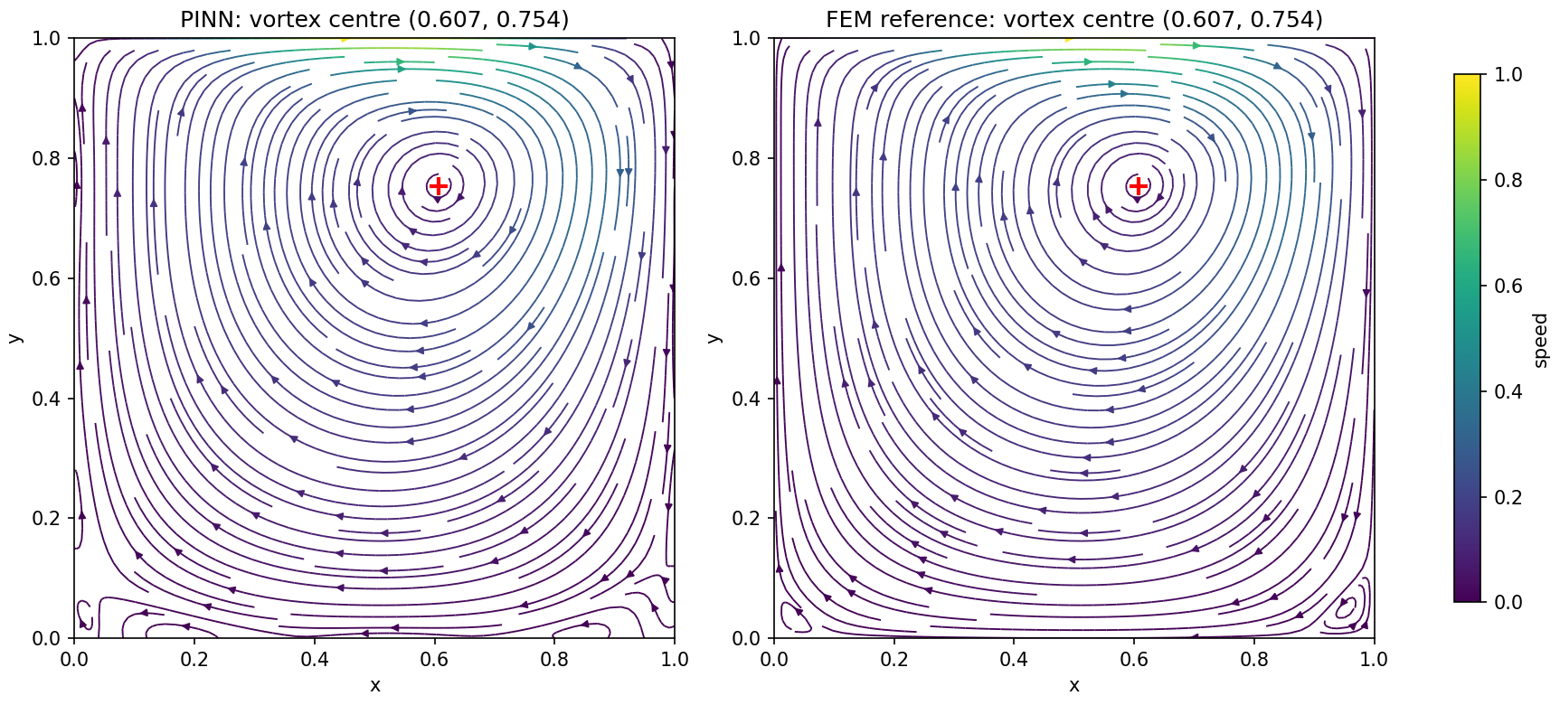
The two panels show the same large clockwise vortex. The fastest fluid, in green, is just under the lid.

The vortex centre is at $(0.6074, 0.7540)$ for the network and $(0.6074, 0.7538)$ for the reference, found on the grid with a parabola through three points. The stream function at the centre is $-0.08365$ against $-0.08369$.

Quantity	Network	Reference	Difference
Vortex centre $x$	0.60740	0.60743	$-3.0\times10^{-5}$
Vortex centre $y$	0.75405	0.75377	$+2.8\times10^{-4}$
$\psi$ at the centre	$-0.08365$	$-0.08369$	$+4.0\times10^{-5}$
Minimum of $u$ on $x = 0.5$	$-0.16349$	$-0.16337$	$-1.2\times10^{-4}$
Height of that minimum	0.46549	0.46615	$-6.6\times10^{-4}$
Maximum of $v$ on $y = 0.5$	0.13870	0.13929	$-5.9\times10^{-4}$
Minimum of $v$ on $y = 0.5$	$-0.19469$	$-0.19535$	$+6.6\times10^{-4}$

The fields

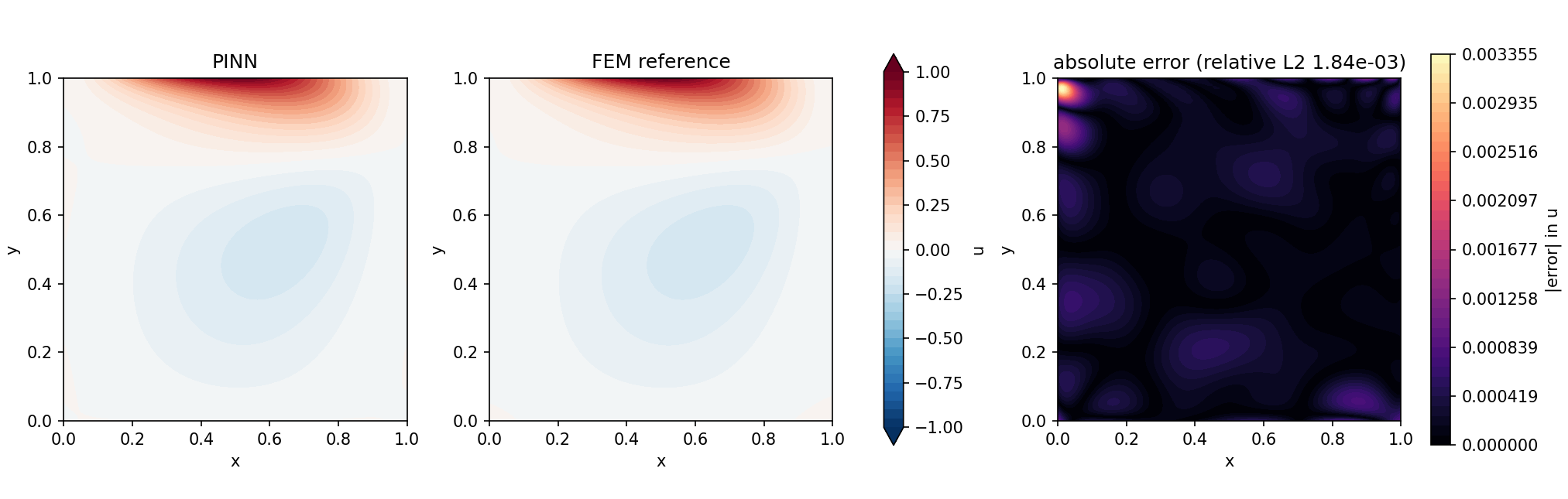
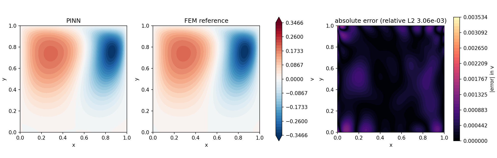
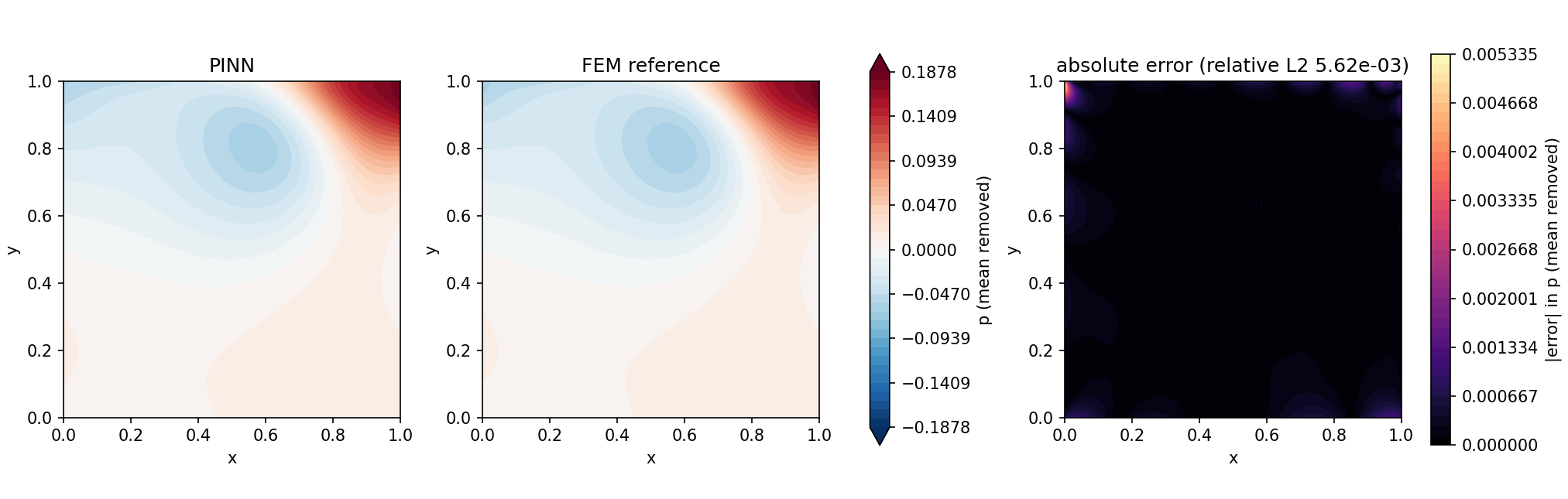
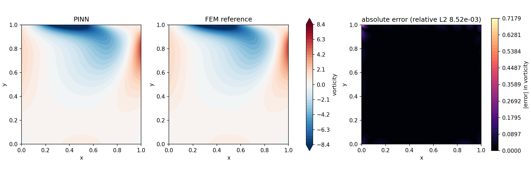
In each figure the left and middle panels share one colour scale, and the error panel has its own, so compare the sizes on the colour bars and not the colours.

The shapes agree to the eye. The horizontal velocity is positive under the lid and negative in the return flow below. The pressure is highest in the top right corner, where the lid drives the fluid into the right wall (up to 0.187), and has a low region around the vortex centre. The vorticity is concentrated under the lid.

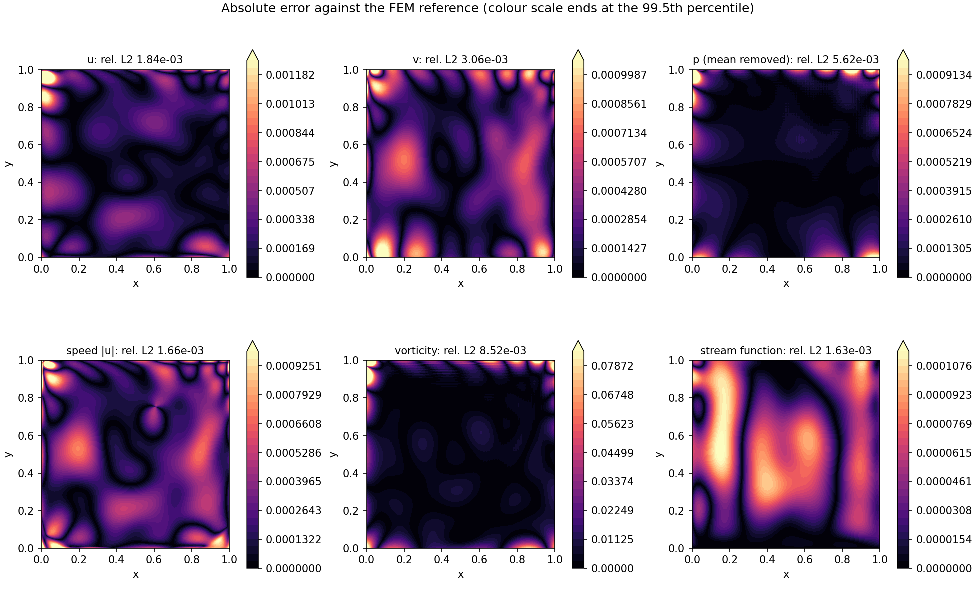
Where the error sits

The error is a smooth pattern spread over the whole cavity, with extra at the walls and especially at the lid corners. Away from the walls (inside $0.05 \le x, y \le 0.95$) the relative L2 errors are $1.99\times10^{-3}$ for $u$, $2.60\times10^{-3}$ for $v$ and $2.79\times10^{-3}$ for $p$. The pressure error is about half as large there as over the whole cavity ($5.62\times10^{-3}$), so a good part of it sits near the walls. The two discs of radius 0.05 around the lid corners cover 0.4 % of the area and hold 7.1 % of the squared velocity error.

$y$ range	RMS velocity error	RMS reference speed	Ratio
0.0 to 0.2	$4.9\times10^{-4}$	$3.5\times10^{-2}$	$1.4\times10^{-2}$
0.2 to 0.4	$3.8\times10^{-4}$	$9.6\times10^{-2}$	$4.0\times10^{-3}$
0.4 to 0.6	$4.2\times10^{-4}$	$1.6\times10^{-1}$	$2.6\times10^{-3}$
0.6 to 0.8	$3.6\times10^{-4}$	$1.9\times10^{-1}$	$1.9\times10^{-3}$
0.8 to 1.0	$5.9\times10^{-4}$	$3.4\times10^{-1}$	$1.7\times10^{-3}$

The absolute error is nearly flat from the floor to the lid, within a factor of 1.6. The ratio is largest near the floor, where the fluid is almost still, so a small absolute error is a larger share of a small speed.

The centreline profiles

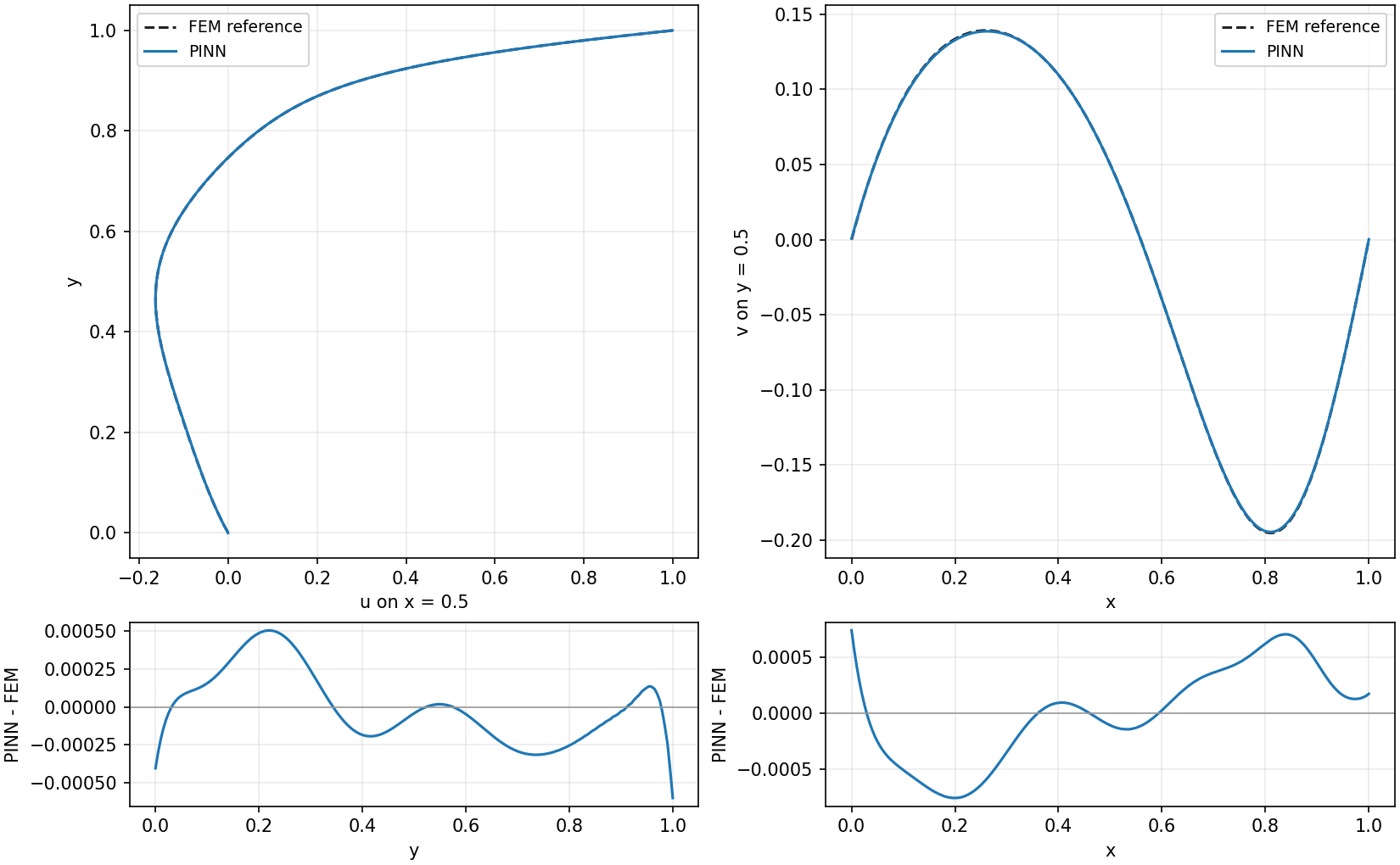
The two curves cannot be told apart at this scale. The differences underneath stay within $\pm 6\times10^{-4}$ for $u$ and $\pm 8\times10^{-4}$ for $v$, and they are smooth.

The lid and the walls

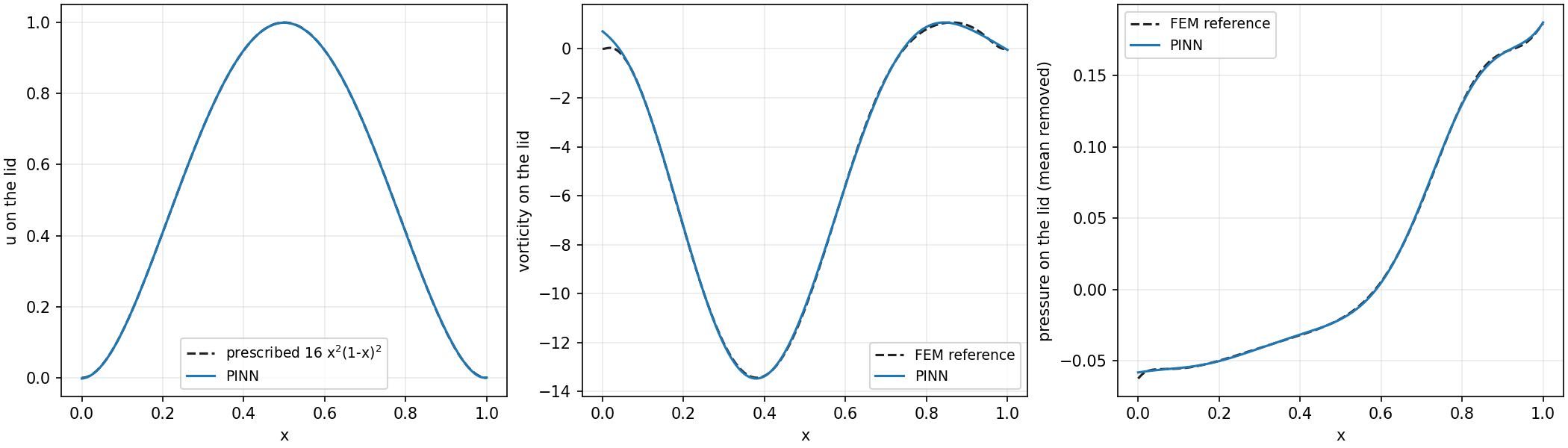
The conditions on the walls are met, not exactly, but to within 0.4 % of the lid speed. The largest $|u|$ on the left, right and bottom walls is $2.9\times10^{-3}$ and the largest $|v|$ is $3.5\times10^{-3}$. On the lid, $u$ differs from $16 x^2 (1 - x)^2$ by an RMS of $5.8\times10^{-4}$, and the largest $|v|$ is $3.5\times10^{-3}$. That largest wall error is at the lid corner $(0, 1)$, the same point where the vorticity error peaks. The vorticity there is about 0.7 for the network where the reference reads about 0. The reference's own vorticity is also least certain on the boundary, so do not read too much into that corner.

The corner eddies

The reference has two tiny eddies in the bottom corners. Their stream function is $1.3\times10^{-6}$ at $(0.035, 0.035)$ in the left corner and $4.8\times10^{-6}$ at $(0.955, 0.050)$ in the right corner, against $-0.0837$ at the primary vortex. The network does not reproduce them. Its stream function differs from the reference by up to $1.2\times10^{-4}$, which is 25 to 90 times larger than the eddies, and the streamlines in the bottom corners of the first figure are not those of the reference.

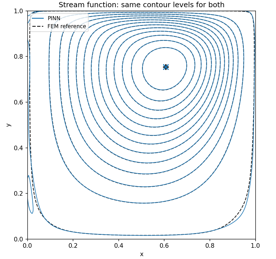
The lines coincide except the outermost ones, near the walls. Those sit at stream-function values of $8\times10^{-6}$ and $-8\times10^{-5}$, far below the vortex's $-0.0837$ and below the network's stream-function error of up to $1.2\times10^{-4}$, so they are the first to differ.

Mass conservation

The net flow across any vertical line should be zero. For the network the integral of $u$ over the full height is at most $1.0\times10^{-4}$ in absolute value for any $x$, and $2.1\times10^{-5}$ at $x = 0.5$. The reference gives at most $2.9\times10^{-5}$. Against the circulation of 0.0837 in the vortex, the network's worst imbalance is 0.12 %.

The equations

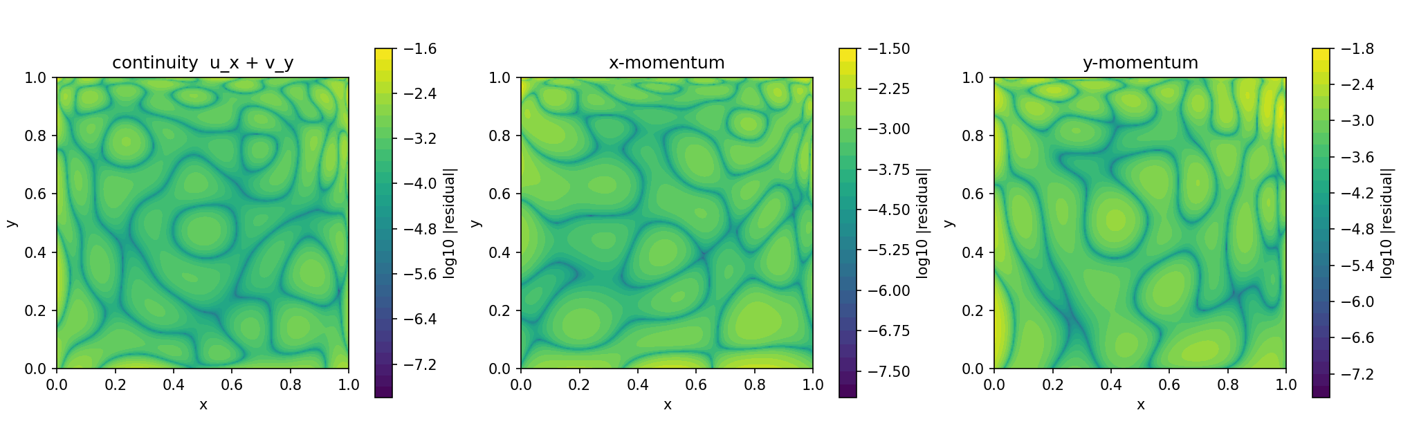
Residual	RMS on the grid	RMS on 10,000 new points	RMS on the training points, from the final loss
continuity	$8.3\times10^{-4}$	$7.5\times10^{-4}$	$7.7\times10^{-4}$
$x$-momentum	$1.2\times10^{-3}$	$1.1\times10^{-3}$	$1.1\times10^{-3}$
$y$-momentum	$1.1\times10^{-3}$	$1.1\times10^{-3}$	$1.1\times10^{-3}$

On the new points the residual is the same as at the training points, so the network satisfies the equations between the training points as well as at them. The residual has no single hot spot in the map. It is a pattern of blobs over the whole cavity, with no single hot spot. The largest values on the new points are $5.5\times10^{-3}$, $1.1\times10^{-2}$ and $1.4\times10^{-2}$.

The training record

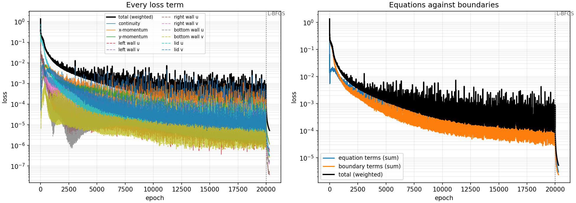
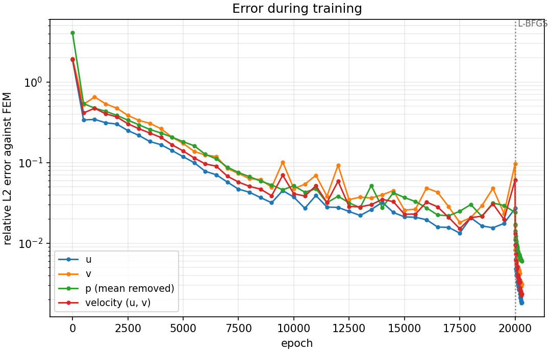
During the 20,000 Adam epochs the total loss fell from 1.35 at the first epoch to a median of $2.4\times10^{-4}$ over the last 500, but with spikes. The largest in those 500 epochs is $2.6\times10^{-3}$, and the last Adam epoch itself, at $8.4\times10^{-4}$, was 3.6 times the median. The velocity error on the snapshots shows the same: 41 % at epoch 500, 14 % at 5,000, 4.1 % at 10,000, then between 1.5 % (epoch 17,500, the best) and 6.1 % (epoch 20,000, a spike) from epoch 15,000 on.

The L-BFGS stage changed the picture. In the first round the total loss fell from $8.4\times10^{-4}$ to $8.2\times10^{-5}$, and by the end of 300 rounds it was $5.3\times10^{-6}$, about 45 times below the Adam median. The velocity error on the snapshot grid fell to 1.3 % after 10 rounds, 0.57 % after 50, 0.51 % after 100 and 0.24 % after 300. At the end the equation terms are 56 % of the loss and the boundary terms 44 %. An error measured at the end of Adam alone would have been between 1.5 % and 6 %, about 6 to 26 times the 0.23 % reported here, so the second stage is not optional for this problem.

Watching it learn

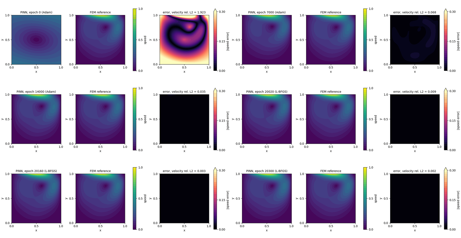
One frame per 500 Adam epochs, then one per 10 L-BFGS rounds. At epoch 2,500 the velocity error is 30 % and the error panel shows a ring around a vortex that is in the wrong place. In the last frames the error panel is black at this scale.

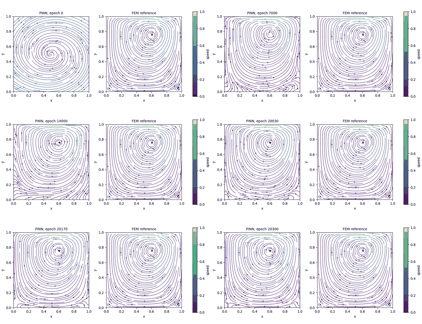
The streamlines of the network close up into the vortex as training goes on. The reference panel does not change.

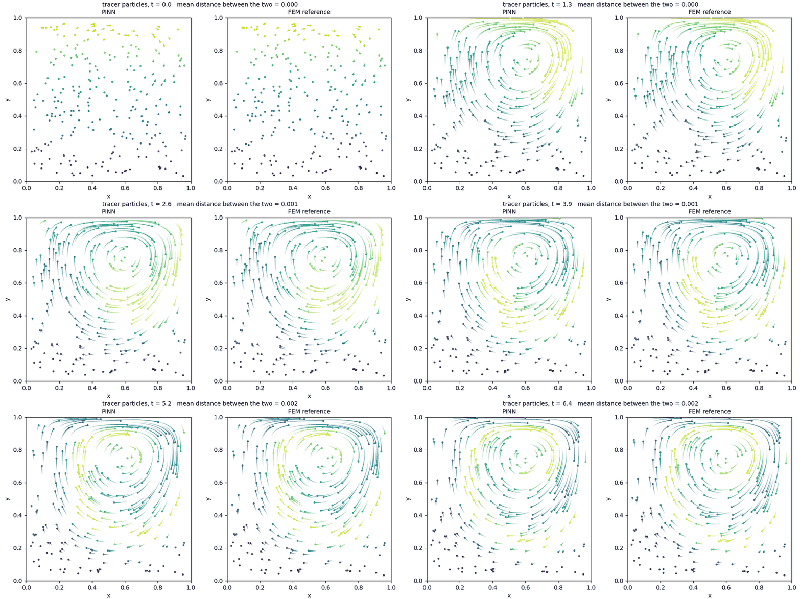
The particles are moved through the steady velocity fields of the trained network and of the reference. At the last frame, $t = 6.4$, the two sets of particles are on average 0.002 apart.

9. What to report

For a PINN result to mean something to a reader, state:

1. The reference, and how you know it is right. Here: Q2–Q1 finite elements on 128 × 128 elements, with third-order convergence on Kovasznay flow and a mesh change of order $10^{-5}$ in velocity.
2. Where you measured. Here a 201 × 201 grid, and 10,000 random points that were not used in training.
3. The relative L2 error of each unknown, plus the RMS and the largest error with its location. For the pressure, say that the mean was removed.
4. The error across the domain. A single number can hide an error that sits at the lid corners or the walls.
5. A physical check. Here, zero net flow across the cavity and the wall conditions. Others are conserved quantities, symmetries and bounds.
6. The residual on new points, next to the training loss.
7. The set-up: network size and activation, the number of points, the loss weights, the optimiser, the epochs, and whether the second stage was used. Report the error after the second stage separately from the error before it.
8. How many runs. This lesson reports one run. Rerun the script several times and give the range, as Poisson in one dimension does.

What this run does not show

• It is one run. Your run will land near these figures, not on them.
• It is one Reynolds number, 100, and one smooth lid. The classic lid and higher Reynolds numbers are harder.
• The network, the points and the loss weights were the Studio defaults, with all weights equal to 1. Nothing was tuned.
• The network does not resolve the two corner eddies. The velocity error is small enough that most uses would not notice, but it is not a statement about those eddies.
• The PINN is not faster than the reference here. The finite element solve took about a minute on a CPU and the network 926 s on a GPU.

10. If something goes wrong

What you see	Likely cause	What to do
Graph check: a complaint about the number of network outputs	The Network block still has one output	Set Network outputs to 3
The pressure map is far from the reference but its pattern is right	A constant was not removed	Subtract the mean of $p$ over the cavity from both fields before comparing
The velocity error is a few per cent (1.5 % to 6 % in our run) and the loss curve is jagged	The run was judged at the end of Adam	Check that the L-BFGS stage ran (--lbfgs-rounds), and compare the error after it
The flow is nearly still, with a very small $u$	The network satisfies the equations with a flow that ignores the lid	Raise the boundary weight, for example --bc-weight 10, and compare the lid profile
The loss is nan or the script stops early	A spike took the weights out of range	Rerun with a smaller LEARNING_RATE
FAILED lines when the figures are made	One figure hit an error	The rest are still written. Run again with --postprocess-only after fixing it
The errors are tens of per cent	Too few epochs, or the L-BFGS stage was skipped	Use the full 20,000 epochs and the second stage

11. Try it yourself

1. Run the script three times. What is the range of the relative L2 error in velocity?
2. Run with --lbfgs-rounds 0. How large is the error at the end of Adam, and how much does it change from one run to the next?
3. Raise the boundary weight with --bc-weight 10. What happens to the error at the walls and to the error in the middle?
4. Double the interior points. Does the residual on new points stay equal to the residual on the training points?
5. Compare the stream-function error of your network with the size of the corner eddies, $1.3\times10^{-6}$ and $4.8\times10^{-6}$. How small would the error have to be to see them?
6. Open the script and find navier_stokes. Remove the continuity term from the loss and run again. What happens to the mass-conservation check?
7. Run python cavity_compare.py --weights weights.npz on your own run and check that it prints the same numbers as the script.

12. Recap

• A flow has several unknowns tied together. The network gets one output for each, and each equation is a loss term.
• The Studio can build and check the problem, but a coupled residual has to be written into the generated script.
• The pressure has no boundary condition and is only defined up to a constant. Remove the mean before comparing.
• The network reached a relative L2 error of 0.23 % in velocity and 0.56 % in pressure on a 201 × 201 grid, with the vortex centre within $3\times10^{-4}$ of the reference.
• The second stage mattered: over its last 5,000 epochs Adam alone stayed between 1.5 % and 6 % velocity error, and L-BFGS brought it to 0.23 %.
• One number is not enough: look at the error across the cavity, check mass conservation and the walls, and compare the residual on new points.

Files: lid_driven_cavity_final.py (training and comparison), cavity_reference.py (the finite element reference and its checks), cavity_compare.py (reproduces the tables from the saved weights, with numpy only), cavity_reference_N128.npz (the reference fields) and cavity_weights_run1.npz (the weights of the run in this lesson).