Read the script
The generated file is long but it has the same nine parts every time, in the same order, each marked by a comment banner. Once you know the parts, you can find any setting you made on the canvas.
You do not have to read the script to use it. But the Lab is only worth trusting if you can read what it wrote, and the file is built to make that possible. Every script has the same layout, whatever the problem.
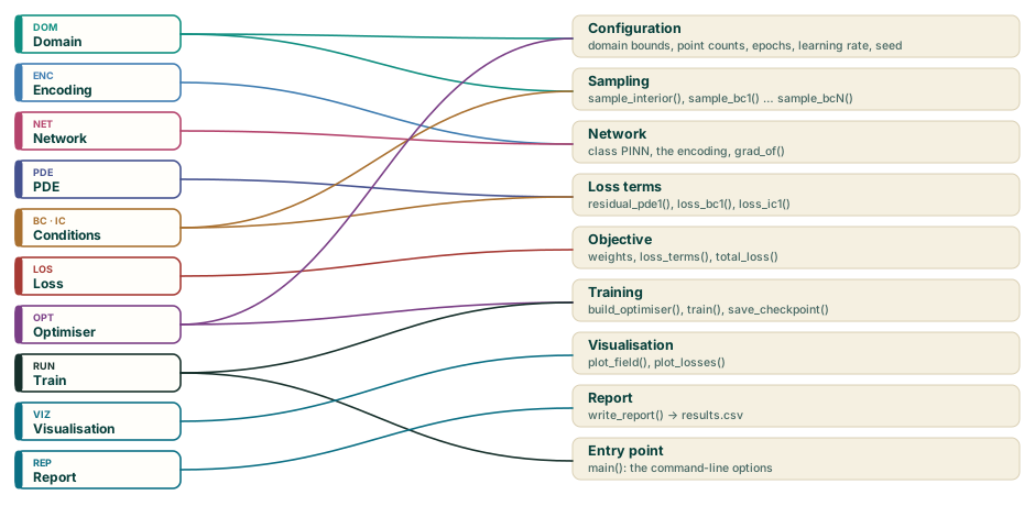
The excerpts below come from a script generated for the 1D Poisson example: $u'' = -\pi^2 \sin(\pi x)$ on $[0, 1]$ with $u = 0$ at both ends. Yours will differ in the details but not in the shape.
The header
The top of the file is a docstring. After the licence note you find a summary of what the graph described.
Geometry    : Line (A 1-D interval [x_min, x_max].)
Coordinates : (x)
Equation    : \nabla^2 u = f(\mathbf{x})
Conditions  : 2 boundary, 0 initial

Run it directly (python this_file.py), or import it and call train().
Command line: --epochs N  --device cpu|cuda  --checkpoint PATH  --no-plots
If the Graph check had any notes when you generated, they follow, under the heading Graph check. A script that surprises you is worth a look at this header first.
1. Configuration
Every number you typed into a block, as a named constant near the top:
TITLE = 'Poisson 1D'
SEED = 0
CHECKPOINT = 'model.pt'

COORDS = ['x']
X_MIN = 0.0
X_MAX = 1.0

N_INTERIOR = 2000
INTERIOR_STRATEGY = 'uniform'

EPOCHS = 5000
LEARNING_RATE = 0.001
LOG_EVERY = 200
RESAMPLE_EVERY = 0
These are the easiest edits to make by hand. Change EPOCHS to 10000, or N_INTERIOR to 4000, and run again. No visit to the Lab is needed.
2. Sampling
Functions that draw the points: sample_interior() for the collocation points inside the domain, and one sample_bc1(), sample_bc2(), … for each boundary. These are the Domain block's output turned into code.
def sample_interior(n: int = N_INTERIOR, strategy: str = INTERIOR_STRATEGY) -> torch.Tensor:
    """Collocation points strictly inside the domain."""
    u = unit_samples(n, 1, strategy)
    x = X_MIN + (X_MAX - X_MIN) * u[:, 0]
    return as_points([x])
Two details are worth knowing. The points are created with requires_grad=True, which is what allows PyTorch to differentiate the network with respect to the coordinates later. And the boundary functions are called anew each time a boundary loss is computed, so the boundary points are redrawn at every epoch, while the interior points are drawn once for the run (unless RESAMPLE_EVERY is above zero). Collocation points in the textbook explains why that distinction matters.
3. Network
The Network block as a PyTorch class, PINN, with the layers you chose:
widths = [width_in] + [40, 40, 40, 40] + [1]
...
layers.append(nn.Linear(widths[i], widths[i + 1]))
if i < len(widths) - 2:
    layers.append(nn.Tanh())
The list [40, 40, 40, 40] is the Hidden layers field, and nn.Tanh() is the Activation. Look at the forward method, too: before the first layer it rescales the coordinates to $[-1, 1]$ using the domain bounds, which is the "input scaling" mentioned in Build the network.
Below the class are two helpers that make a PINN possible.
def grad_of(y, pts):
    """d y / d pts, as one tensor with a column per coordinate."""
    ...
    gradient = torch.autograd.grad(
        y, pts, grad_outputs=torch.ones_like(y), create_graph=True, retain_graph=True, allow_unused=True
    )[0]
grad_of asks PyTorch's automatic differentiation for the derivative of the network's output with respect to the input points. create_graph=True is the important part. It keeps the derivative itself differentiable, so you can differentiate it again for a second derivative. This one function is what the textbook's chapter on automatic differentiation turns into code.
4. Loss terms
One function per term of the loss. This is where the PDE and BC / IC blocks live. For Poisson:
def residual_pde1(pts):
    """Interior residual of the poisson equation; zero when it is satisfied."""
    u = field(pts, 0)
    x = pts[:, 0:1]
    g1 = grad_of(u, pts)
    u_x = g1[:, 0:1]
    g2_x = grad_of(u_x, pts)
    u_xx = g2_x[:, 0:1]
    f = ((-(math.pi ** 2.0)) * torch.sin((math.pi * x)))
    return (u_xx) - f
Read it line by line. u is the network's output. u_x is its first derivative, found by calling grad_of once; u_xx is the derivative of that, found by calling it again. f is your formula, -pi**2*sin(pi*x), translated into PyTorch. The returned value, $u_{xx} - f$, is the residual: zero when the equation is satisfied.
A boundary condition is simpler:
def loss_bc1():
    """Dirichlet condition on BC1."""
    pts, normals = sample_bc1()
    u = field(pts, 0)
    target = 0.0
    return reduce_term(u - target)
It draws its points, evaluates the network there and measures how far the value is from the target. reduce_term is the mean square, that is the Term norm you chose in the Loss block.
5. Objective
Here the loss weights from the Loss block are applied. The dictionary of group weights and a function that sums every term:
GROUP_WEIGHTS = {"pde": 1.0, "bc": 1.0, "ic": 1.0}

def total_loss(pts):
    terms = loss_terms(pts)
    total = torch.zeros((), device=DEVICE)
    for name, value in terms.items():
        group = TERM_GROUPS.get(name, "pde")
        total = total + balancer.weights.get(group, 1.0) * TERM_SCALES.get(name, 1.0) * value
    return total, terms
The sum is exactly the formula on Balance the loss. If you set per-boundary weights, they appear in TERM_SCALES, one number per term.
6. Training
build_optimiser() makes the optimiser from the Optimiser block, and train() is the loop. Its core is five lines:
optimiser.zero_grad(set_to_none=True)
total, terms_now = total_loss(pts)
if total.requires_grad:
    total.backward()
optimiser.step()
Forget the old gradients, compute the loss, differentiate it with respect to the weights (backward), and move the weights one step. Everything else in train() records the history and prints progress. save_checkpoint() then writes the weights and the history. This is gradient descent in its entirety.
Where the seed is set
train() begins with torch.manual_seed(SEED). The network, however, is built earlier, when the file is first loaded, so its starting weights are not governed by that seed. Two runs of the same script can start from different weights. If you need the same starting weights every time, put torch.manual_seed(0) just before the line net = PINN().to(DEVICE).
7 and 8. Visualisation and Report
plot_field() and plot_losses() draw the pictures, each saved by a small helper called _finish. write_report() writes the table. If you left the Visualisation or Report block out, these parts are simply not in the file.
9. The entry point
The last part is main(), which reads the command-line options, calls train(), saves the checkpoint, draws the figures and writes the table, in that order. The if __name__ == "__main__": line at the bottom means that importing the file does nothing, so you can use its functions elsewhere (see Run the script).
Making a change by hand
The script is yours to edit. Two good habits.
- Prefer changing the notebook for anything structural: a different equation, a different geometry, an extra boundary condition. The Lab regenerates the whole file correctly, and your canvas stays the record of what you did.
- Edit the file for quick experiments: the constants in section 1, an extra
print, a different plot. Keep a copy of the generated original beside it so you can compare.
A good test of a change is the residual: after any edit, call residual_pde1(sample_interior()) and look at its size. A residual that is small only at the training points and large elsewhere means the network has learned the points, not the equation.
Chapter 4 is finished. In chapter 5 you put everything together, starting with a notebook built from an empty canvas.