Define the domain
The Domain block says where the problem lives, where its edges are, how many points to sample, and whether time is part of it.
Everything else takes its coordinates from the Domain, so you place it first. It has no inputs. Its outputs feed the PDE (the inside), the boundary conditions (the edges), the initial condition (if time is on) and the Network (the coordinates).
1. Choose the geometry
Set Geometry type to one of three shapes. The shape decides which numbers you enter, and how many boundaries the block has.
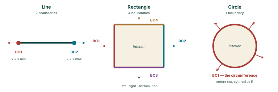
| Geometry | You enter | Boundaries |
|---|---|---|
| Line | x min, x max | BC1 at x = x min, BC2 at x = x max |
| Rectangle | x min, x max, y min, y max | BC1 left, BC2 right, BC3 bottom, BC4 top |
| Circle | Centre x, Centre y, Radius | BC1, the circumference |
The ends must be in order: x max must be greater than x min, and the radius must be greater than zero. If not, the Graph check says, for example, Domain: x_min must be smaller than x_max (currently 1 and 0).
Your screenshot · the Domain block set to Rectangle, with the four boundary ports visible on the block and the Geometry group open in the panel.
2. Detect the boundaries
A boundary is not something you name. The geometry has its boundaries, and the Lab reports them. Press Detect boundaries and the panel prints a line such as:
Detected 4 boundaries: BC1 (x = x_min (left)), BC2 (x = x_max (right)), BC3 (y = y_min (bottom)), BC4 (y = y_max (top))
Each boundary is also an output port on the block, labelled BC1, BC2, and so on. That is where you attach a boundary-condition block in the next step. Hover over a port to see which edge it is.
3. Sample the points
A PINN checks the equation at a finite set of points, called collocation points (see the textbook). Three groups of settings control them.
Interior points are the points inside the domain where the PDE must hold.
- Interior points: how many. The default is 2000. A larger number is more accurate and slower.
- Interior distribution: how they are placed. Uniform random is the usual default. Regular grid spaces them evenly, and for a 2-D domain the Lab rounds the count to the nearest square (2000 becomes 45 × 45 = 2025). Latin hypercube and Sobol sequence spread random points more evenly than plain uniform, and can converge faster on smooth solutions with fewer points.
Boundary points are the points on each edge where a condition must hold.
- Default boundary points: how many per boundary (default 80).
- Points per boundary: a table with one row per boundary, each with its own Points and Distribution. Leave a row alone to inherit the default. Give extra points only to the edges where the solution actually changes quickly.
Sampling seed. This field is stored in the notebook, but the generated script takes its seed from the Train block's Random seed, so set the seed there.
4. Switch on time
Tick Time dimension if the equation changes in time (heat, wave, Burgers, advection, diffusion-reaction). Three things happen:
- t initial and t final appear (defaults 0 and 1), plus Time points and Initial points.
tbecomes the last coordinate, and the Network gains one input.- The block grows an Initial output, for the initial-condition block.
Initial points is how many points sample the t = t initial surface. The interior and boundary points are drawn over space and time together, so Interior points is what sets how densely time is sampled. Time points is written into the configuration at the top of the script but is not used to place points.
Leave time off for steady problems (Poisson, Laplace, steady conduction, Helmholtz). The Graph check complains if the equation and the time setting disagree.
5. Preview what you have set
Plot geometry and points draws the domain, the sampled interior points, and each boundary in its own colour with its outward normals. It is a quick way to catch a boundary on the wrong side, or too few points on an edge. A second press hides it. The preview uses a fixed random seed, so it does not reshuffle every time you type a number.
Your screenshot · the Plot geometry and points preview for a rectangle, showing interior points and four coloured edges.
Checklist
- The geometry is the one in your problem, and the bounds are in order.
- Every boundary you will constrain has an output port.
- Time is on exactly when the equation has a time derivative.
- The number of interior points is generous enough for your equation; you can raise it later.
Next: choosing the equation.